Review

Pharmacology of doping agents—mechanisms promoting muscle hypertrophy

  • Doping with performance enhancing substances in professional andamateur sports has increasingly gained awareness. Furthermore, not only thenumber but also the variety of substances detected in sports has increased.Intending muscle growth, anabolic androgenic steroids (AAS) have beencomplemented by selective androgen receptor modulators (SARMs), β2-adrenergicagonists, estrogen receptor (ER) β agonists and peptide-hormones like growthhormone (GH), insulin-like growth factor-1 (IGF-1) and insulin. However, withrespect to therapeutic use, drugs which increase anabolic actions in the bodyare highly desired for treatment of cachexia, sarcopenia, etc.
    The aim of the following review is to elaborate on the agents’similarities and differences in mechanisms inducing muscle hypertrophy whilegiving an overview of the relevant signalling cascades. In addition to that,potential agents for treatment of catabolic diseases are identified.Information, onwhich this paper is based on, hasbeen collected from various publications which have been published inhigh-quality scientific journals.
    The insight obtained has shown that signalling pathways mediatinggenomic actions of steroids have already been well-characterised, while thereis still need for further research on the mechanisms of non-genomicactions and downstream pathways as well as on those of SARMs and β2-adrenergicagonists’ action. A new and promising target is the estrogen receptor β. Theuse of ER-β agonists, which are proposed to activate anabolic mechanismsindependently from androgen receptor activation, may prevent the non-desiredandrogenic effects, which are associated with AAS administration. Thus, theymay be considered a promising alternative for treatment of diseases, whichcause loss of muscle mass and cachexia. In this context, phytoecdysteroids,such as ecdysterone etc, are considered as an interesting class of substances,where further investigations are highly desired. Furthermore, some peptidehormones also promote muscle hypertrophy. The signalling mechanisms of growthhormone, IGF-1 and insulin are summarised. Finally, the potential of myostatininhibition is discussed.

    Citation: Maria Kristina Parr, Anna Müller-Schöll. Pharmacology of doping agents—mechanisms promoting muscle hypertrophy[J]. AIMS Molecular Science, 2018, 5(2): 131-159. doi: 10.3934/molsci.2018.2.131

    Related Papers:

    [1] Mengya Huang, Anji Yang, Sanling Yuan, Tonghua Zhang . Stochastic sensitivity analysis and feedback control of noise-induced transitions in a predator-prey model with anti-predator behavior. Mathematical Biosciences and Engineering, 2023, 20(2): 4219-4242. doi: 10.3934/mbe.2023197
    [2] Frédérique Billy, Jean Clairambault, Franck Delaunay, Céline Feillet, Natalia Robert . Age-structured cell population model to study the influence of growth factors on cell cycle dynamics. Mathematical Biosciences and Engineering, 2013, 10(1): 1-17. doi: 10.3934/mbe.2013.10.1
    [3] Maria Vittoria Barbarossa, Christina Kuttler, Jonathan Zinsl . Delay equations modeling the effects of phase-specific drugs and immunotherapy on proliferating tumor cells. Mathematical Biosciences and Engineering, 2012, 9(2): 241-257. doi: 10.3934/mbe.2012.9.241
    [4] J. M. Cushing . Nonlinear semelparous Leslie models. Mathematical Biosciences and Engineering, 2006, 3(1): 17-36. doi: 10.3934/mbe.2006.3.17
    [5] Jiayin Song, Yue Zhao, Zhixiang Chi, Qiang Ma, Tianrui Yin, Xiaopeng Zhang . Improved FCM algorithm for fisheye image cluster analysis for tree height calculation. Mathematical Biosciences and Engineering, 2021, 18(6): 7806-7836. doi: 10.3934/mbe.2021388
    [6] Md Masud Rana, Chandani Dissanayake, Lourdes Juan, Kevin R. Long, Angela Peace . Mechanistically derived spatially heterogeneous producer-grazer model subject to stoichiometric constraints. Mathematical Biosciences and Engineering, 2019, 16(1): 222-233. doi: 10.3934/mbe.2019012
    [7] Shingo Iwami, Shinji Nakaoka, Yasuhiro Takeuchi . Mathematical analysis of a HIV model with frequency dependence and viral diversity. Mathematical Biosciences and Engineering, 2008, 5(3): 457-476. doi: 10.3934/mbe.2008.5.457
    [8] Lina Hao, Meng Fan, Xin Wang . Effects of nutrient enrichment on coevolution of a stoichiometric producer-grazer system. Mathematical Biosciences and Engineering, 2014, 11(4): 841-875. doi: 10.3934/mbe.2014.11.841
    [9] Lin Chen, Xiaotian Wu, Yancong Xu, Libin Rong . Modelling the dynamics of Trypanosoma rangeli and triatomine bug with logistic growth of vector and systemic transmission. Mathematical Biosciences and Engineering, 2022, 19(8): 8452-8478. doi: 10.3934/mbe.2022393
    [10] Jian Zu, Wendi Wang, Bo Zu . Evolutionary dynamics of prey-predator systems with Holling type II functional response. Mathematical Biosciences and Engineering, 2007, 4(2): 221-237. doi: 10.3934/mbe.2007.4.221
  • Doping with performance enhancing substances in professional andamateur sports has increasingly gained awareness. Furthermore, not only thenumber but also the variety of substances detected in sports has increased.Intending muscle growth, anabolic androgenic steroids (AAS) have beencomplemented by selective androgen receptor modulators (SARMs), β2-adrenergicagonists, estrogen receptor (ER) β agonists and peptide-hormones like growthhormone (GH), insulin-like growth factor-1 (IGF-1) and insulin. However, withrespect to therapeutic use, drugs which increase anabolic actions in the bodyare highly desired for treatment of cachexia, sarcopenia, etc.
    The aim of the following review is to elaborate on the agents’similarities and differences in mechanisms inducing muscle hypertrophy whilegiving an overview of the relevant signalling cascades. In addition to that,potential agents for treatment of catabolic diseases are identified.Information, onwhich this paper is based on, hasbeen collected from various publications which have been published inhigh-quality scientific journals.
    The insight obtained has shown that signalling pathways mediatinggenomic actions of steroids have already been well-characterised, while thereis still need for further research on the mechanisms of non-genomicactions and downstream pathways as well as on those of SARMs and β2-adrenergicagonists’ action. A new and promising target is the estrogen receptor β. Theuse of ER-β agonists, which are proposed to activate anabolic mechanismsindependently from androgen receptor activation, may prevent the non-desiredandrogenic effects, which are associated with AAS administration. Thus, theymay be considered a promising alternative for treatment of diseases, whichcause loss of muscle mass and cachexia. In this context, phytoecdysteroids,such as ecdysterone etc, are considered as an interesting class of substances,where further investigations are highly desired. Furthermore, some peptidehormones also promote muscle hypertrophy. The signalling mechanisms of growthhormone, IGF-1 and insulin are summarised. Finally, the potential of myostatininhibition is discussed.


    At the global scale, the hydrologic cycle is the endless recirculatory process of water movement within the atmosphere and across the Earth's surface. This cycle comprises three primary processes: evaporation, condensation, and precipitation. The Earth's hydrologic cycle is driven and sustained by various natural sources and processes, including oceans, lakes, ponds, forests, sunlight, and atmospheric dynamics. Sunlight facilitates the evaporation of water from major water bodies, such as oceans, lakes, and ponds, forming water vapor that ascends into the atmosphere. Additionally, forest, trees, plants, and agricultural crops contribute to atmospheric moisture through the transpiration process [1,2]. When water vapor reaches to the atmosphere, it undergoes the process of condensation and aggregation to form vapor clouds. These vapor clouds convert into raindrops, which eventually precipitate back to the Earth's surface under the influence of gravity. This cyclical exchange of water between the Earth's surface and atmosphere, mediated by evaporation, transpiration, condensation, and precipitation, ensures the continuity of the global hydrologic cycle.

    Water is a vital resource for sustaining human life and underpins ecosystem's services crucial for maintaining ecosystems. Human population relies on the hydrologic cycle to fulfill their demand of fresh water, yet disrupts it through their unsustainable development activities. Based on an analysis of a global data set of large lakes and rivers, [3] concluded that transpiration recycles approximately 62,000 $ \pm $ 8000 Km$ ^3 $ of water annually to the atmosphere. It is also observed that evapotranspiration via forest trees plays a major role in regulating fluxes of atmospheric moisture, but human–induced large–scale deforestation weakens regional moisture recycling and leads to rainfall suppression [4,5,6]. On a global scale, a massive deforestation has been done for the construction of buildings, roads, highways, agricultural land, etc., and the root cause of this is overpopulation, which demands space for living, more food production for survival, and rapid development [7]. Research studies show that, before the development of human civilization, the Earth's surface was covered by approximately 60 million square kilometers of forest. However, due to extensive deforestation and land-use changes, the forest cover has been reduced to approximately 40 million square kilometers [8]. As of 2012, approximately 20$ \% $ of the Amazon rainforest had been transformed into agricultural areas, pasture lands, and other human–dominated landscapes [9,10,11]. Environmental studies show that several anthropogenic activities have significantly altered the ecological dynamics of forest ecosystems, which lead to disruption in forming vapor clouds and rainfall patterns. According to an analysis conducted by Smith et al. [12], the impact of forest loss between 2003 and 2017 on precipitation within a 200-km area was quantified and showed that a 1$ \% $ increase in forest loss was associated with a reduction in monthly precipitation of 0.25 $ \pm $ 0.1 mm. A precipitationshed moisture tracking framework indicates that the forested regions in Rondonia (Brazilian Amazon) contribute to approximately 48$ \% $ of the annual rainfall on average [13,14].

    The reduction in evapotranspiration due to deforestation, disturbance in the formation of vapor clouds due to less evaporation or a deteriorated condensation-nucleation process for forming raindrops are all associated with population growth and its developmental activities. The expansion in settlements of growing human population has led to the loss of small water bodies, such as ponds and open water sources, which significantly diminishes the evaporation from these surfaces to the global water cycle [15]. It is estimated that over the last century, damaged ecosystems have lost approximately 37,000 Km$ ^3 $ of freshwater from their small hydrologic cycles, and in the last 20 years, deforestation and urbanization have caused an annual fresh water loss of 760 Km$ ^3 $ [16].

    Alongside this, larger aquatic systems, including lakes and ponds, are increasingly affected by nutrient enrichment (eutrophication), promoting excessive growth of algae and macrophytes that form dense mats of pollution over the water surface [17]. This algal proliferation inhibits evaporation by reducing the exposed surface area of water. Additionally, urbanization and infrastructure expansion, such as the construction of residential complexes and roads/highways, and extensive coverage of land with impermeable materials like concrete and cement, have drastically reduced ground evaporation [18,19].

    Besides water pollution, anthropogenic activities also cause atmospheric pollution, which affects the condensation-nucleation of vapor clouds and the agglomeration of clouds to form raindrops. Thus, the research studies reflect the negative impacts of increased human activities on hydrologic processes and the natural balance of the Earth's water cycle [20].

    Some modeling researches have been carried out by the researchers to address the problem of deforestation caused by human population and industrialization [21,22]. It is emphasized in these studies that the forestry resources may become very low because of large population pressure and its augmented industrialization, even if the population growth is partially dependent on forestry resources. In 2020, Lata and Misra [23] conducted a modeling study to assess the impact of forestry trees on precipitation patterns, concluding that tree species with a higher intrinsic growth rate contribute positively in enhancing rainfall. Based on the experimental and observational studies, it is noticed that the growing human population affects the dynamics of forest trees, rainfall, as well as the hydrologic cycle [24,25,26]. Further, some modeling studies to analyze the effects of human population and its augmented pollution on rainfall have been conducted, as discussed in [27,28] and the references therein. The results show that factors, such as urbanization, industrialization, and atmospheric pollutants negatively impact the clouds' formation, and thus rainfall. To address the challenges associated with deforestation, conservation of forest resources [23], atmospheric pollution [29,30], rainfall suppression [31], and artificial rainfall [32,33,34], various modeling studies have been undertaken aiming to improve precipitation patterns and alleviate environmental impacts, which can be studied in the cited studies and the references therein.

    For the continuous process of the hydrologic cycle, transpiration and evaporation are the important factors. The forest determines the recycling of water by releasing the water vapor into the atmosphere via their stomata (microscopic pores located on leaves and other tree surfaces). In addition to transpiration, evaporation from open water bodies, soils, and other wet surfaces significantly contributes to atmospheric water vapor, leading to cloud formation, and thus raindrops. However, recent trends reveal a decline in wet surfaces, deforestation, depletion of open water sources, and increased concentration of aerosols. These changes are driven by increasing human population and associated developmental activities, such as constructing impervious surfaces, expanding urban areas, industrial air and water pollution, etc.

    The dynamics of rainfall as well as the hydrologic cycle, influenced by environmental fluctuations, can be effectively analyzed using nonlinear ordinary and stochastic differential models. Therefore, in this study, an integrated investigation of the effects of human population on forestry trees' density, cloud formation, and rainfall dynamics is undertaken. Thus, the present study develops and analyzes a novel mathematical model for the assessment of the hydrologic cycle under the combined influences of human population and forestry trees.

    From the above literature review, we observe that forest trees and the human population play a significant role in the regulation of the water cycle. Therefore, to understand the dynamic relationship between rainfall, forest trees, and human population, we introduce a four-dimensional nonlinear mathematical model involving the density of forest trees, the density of human population, and the densities of vapor clouds and raindrops as the dynamic variables, representing them by $ F(t) $, $ N(t) $, $ V(t) $, and $ R(t) $ at any time $ t $, respectively.

    We establish the base of our model on several key speculations, which are as follows:

    ● Forest trees grow logistically having intrinsic growth rate $ s_0 $ and carrying capacity $ s_0/s_1 $. Here, $ s_1 $ represents an intra-specific competition coefficient, which encapsulates the effects of resource limitations, including sunlight, water, land, and nutrients on the forestry trees [35]. Furthermore, the growth of the human population is also modeled by a logistic growth equation characterized by an intrinsic growth rate $ r_0 $ and carrying capacity defined as $ r_0/r_1 $. Here, $ r_1 $ represents an intra-specific competition coefficient, which arises due to the constraints imposed by limited food, water, and land resources [36].

    ● Moreover, it is observed that the increasing human population cuts down the forest trees for resource needs, like the expansion of cities and towns, construction of highways, housing, roads, and industries, agricultural purposes, logging for wood products and fuelwood, etc. [8,9,11]. Therefore, we assume that the per capita density of forest trees depletes at a rate $ \alpha_1 N $ caused by harvesting for the survival of the human population. Consequently, the density of the human population increases proportionally to the depletion of the density of forest trees, represented by the term $ \pi_1 \alpha_1 N F $, where $ \pi_1 $ is the proportionality constant and $ \pi_1 \in (0, 1) $.

    ● Vapor clouds are naturally formed in the atmosphere at a constant rate $ Q $; however the reduction in the formation of vapor clouds is observed due to reduced evaporation. Observational studies show that the extinction of open water resources, such as ponds, lakes, rivers, etc., and eutrophied/polluted water sources, are the major causes for water evaporation reduction, which results in less formation of vapor clouds [15,16,17]. Along with this, the development of roads, industrialization, urbanization, etc., covers most of the land with concrete/cement in cities to fulfill the demand of the increasing human population [18,19]. This significantly reduces the evaporation of water from the ground. Also, the atmospheric pollutants, released due to the anthropogenic activities, deteriorate the condensation-nucleation process to form the clouds [28]. Therefore, we assume that the human population significantly reduces the natural formation rate of vapor clouds ($ Q $) following a Holling type Ⅱ functional response $ \frac{\theta N}{m+N} $. Here, $ \theta $ represents the reduction coefficient associated with the formation of vapor clouds due to human population, and $ m $ represents the half saturation constant.

    ● It is observed that water vapor condenses around atmospheric aerosols and creates microscopic cloud droplets. These droplets grow by colliding and merging with others within the cloud. When these cloud droplets become too heavy to float in the atmosphere, they fall on the land as rainfall [37,38,39]. So, we assume that the natural depletion of vapor clouds occurs at a rate $ \delta V $ because of their conversion into raindrops. Consequently, the raindrops are naturally formed in the atmosphere due to the conversion of vapor clouds into raindrops at a rate $ \lambda \delta V $, and the natural depletion of rainfall occurs at a rate $ \delta_1 R $. Here, $ \lambda $ is a proportionality constant, such that $ \lambda \in (0, 1) $. It is observed that trees recharge atmospheric moisture, contributing to vapor clouds' formation by evapotranspiring [40,41,42]. We represent this contribution by the term $ \nu F $, where $ \nu $ is the formation rate of vapor clouds due to transpiration from forest trees.

    ● Studies depict that the growth of forest trees influences and is being influenced by rainfall. The forest trees absorb the rain water through their roots, stems, leaves, etc., as water is essential for photosynthesis, nutrient transport, and cellular functions. So, we assume that the density of raindrops depletes at a rate $ \gamma RF $, and the density of forest trees increases proportionally to this depletion rate. We represent this growth of forest trees by the term $ \eta\gamma RF $. Here, $ \eta $ is a proportionality constant and $ \eta \in (0, 1) $.

    The above discussed assumptions are now systematically expressed in the form of nonlinear ordinary differential equations. The given equations depict the rate of change of our considered dynamical variables with respect to time and provide a mathematical representation of the interactions among various factors that influence the hydrological cycle:

    $ dFdt=s0Fs1F2α1NF+ηγRF,dNdt=r0Nr1N2+π1α1NF,dVdt=Q(1θNm+N)δV+νF,dRdt=λδVδ1RγRF,
    $
    (2.1)

    with initial conditions $ F(0) \geq 0 $, $ N(0) \geq 0 $, $ V(0) > 0 $, and $ R(0) > 0 $.

    A visual representation of all the discussed assumptions is framed in a schematic diagram, Figure 1. The diagram represents the main hydrological factors, along with associated variables and parameters, involved in modeling the system (2.1). Further, a table consisting of the description of all parameters with their numerical values and units is presented in Table 1.

    Figure 1.  Schematic representation of the interplay between all dynamic variables and parameters involved in modeling the process of the hydrologic cycle as in model system (2.1).
    Table 1.  Numerical values of parameters with their description.
    Parameter Description Numerical value Unit
    $ s_0 $ Intrinsic growth rate of forest trees 0.2 year$ ^{-1} $
    $ s_1 $ Depletion rate of forest trees due to intra-specific competition 2.0 $ \times $ 10$ ^{-5} $ trees$ ^{-1} $ year$ ^{-1} $
    $ \alpha_1 $ Depletion rate of forest trees due to harvesting by the human population 1.0 $ \times $ 10$ ^{-8} $ person$ ^{-1} $year$ ^{-1} $
    $ \eta $ Growth of forest trees due to rainfall, $ \eta \in (0, 1) $ 0.0476 trees mm$ ^{-1} $
    $ \gamma $ Depletion rate of raindrops due to its absorption by forest trees 2.7203 $ \times $ 10$ ^{-7} $ trees$ ^{-1} $year$ ^{-1} $
    $ r_0 $ Intrinsic growth rate of the human population 0.08 year$ ^{-1} $
    $ r_1 $ Decay rate of the human population due to intra-specific competition 1.0 $ \times $ 10$ ^{-5} $ person$ ^{-1} $year$ ^{-1} $
    $ \pi_1 $ A proportionality constant representing the growth of the human population due to harvesting of the forest for their survival 0.01 person trees$ ^{-1} $
    $ Q $ Natural formation rate of vapor clouds 285 mm year$ ^{-1} $
    $ \theta $ A reducing factor in the natural formation of vapor clouds due to anthropogenic activities 0.3 -
    $ m $ Half saturation constant due to the human population 50 person
    $ \delta $ Natural depletion rate of vapor clouds 0.1 year$ ^{-1} $
    $ \nu $ Formation rate of vapor clouds due to transpiration from forest trees 2.044 $ \times $ 10$ ^{-4} $ mm trees$ ^{-1} $ year$ ^{-1} $
    $ \lambda $ Conversion of vapor clouds into raindrops, $ \lambda \in (0, 1) $ 0.8 -
    $ \delta_1 $ Natural depletion rate of raindrops 0.13 year$ ^{-1} $

     | Show Table
    DownLoad: CSV

    Now, to analyze the proposed model system (2.1), we apply the qualitative theory of differential equations as it provides insights into the long-term behavior of the nonlinear model system and extracts meaningful information about the dynamics of the system.

    Lemma 1. The bounded set

    $ Ω={(F,N,V,R)R4+: 0F+V+R(s0+ν)2+4s1Q4s1min{δ(1λ),δ1}=:ρm,  0Nr0+π1α1ρmr1},
    $
    (2.2)

    encloses the region of attraction for the model system (2.1) for all its solutions in the interior of the positive orthant. The proof of this lemma can be followed from [43,44].

    To evaluate the equilibrium solutions of the model system (2.1), we equate the time derivative of all the dynamical variables to zero [45]. For this, we have the following set of algebraic equations:

    $ F(s0s1Fα1N+ηγR)=0,
    $
    (3.1)
    $ N(r0r1N+π1α1F)=0,
    $
    (3.2)
    $ Q(1θNm+N)δV+νF=0,
    $
    (3.3)
    $ λδVδ1RγRF=0.
    $
    (3.4)

    From the above set of algebraic equations, four feasible equilibrium solutions of the formulated model system (2.1) are obtained, which are as follows:

    $ {\rm{i}}. $ At $ F = 0 $ and $ N = 0 $, we obtain a boundary equilibrium $ E_0\left(0, 0, \frac{Q}{\delta}, \frac{\lambda Q}{\delta_1}\right) $, which is always feasible. From this equilibrium solution, the dynamics of vapor clouds and raindrops can be studied, while forestry trees and the human population act as bystanders in the hydrological process. This represents the functioning of the hydrological cycle including natural formation of vapor clouds through evaporation, and the condensation-nucleation of clouds into raindrops, despite the participation of forest trees (which contribute in forming vapor clouds through the transpiration process) and the human population (affecting the natural formation rate of vapor clouds and density of forest trees) in the system.

    $ {\rm{ii}}. $ At $ F = 0 $ and $ N \neq 0 $, we obtain an equilibrium, represented by $ E_1 $ as $ E_1 \left(0, \frac{r_0}{r_1}, \frac{Q}{\delta}\left(\frac{m r_1 + (1-\theta)r_0}{m r_1 + r_0} \right), \frac{\lambda Q}{\delta_1} \left(\frac{m r_1 + (1-\theta)r_0}{m r_1+r_0} \right) \right) $, which is feasible without any condition. In analyzing this equilibrium solution, we consider the impact of the human population on the dynamics of vapor clouds and raindrops, whereas the impact of transpiration from forestry trees remains excluded on other dynamical variables.

    This reflects the process of the hydrologic cycle, where the influence of forestry trees, such as their harvesting for human survival, and transpiration for regulating atmospheric moisture, remains uninvolved. However, other atmospheric processes, such as evaporation from open land water resources, condensation, and the nucleation of vapor clouds to form raindrops, persist to regulate the dynamics of the hydrologic cycle.

    $ {\rm{iii}}. $ At $ F \neq 0 $ and $ N = 0 $, we obtain an equilibrium, represented by $ E_2 $ given as $ E_2\left(\hat{F}, 0, \hat{V}, \hat{R}\right) $, provided $ \hat{F} > s_0/s_1 $. By evaluating the Eqs (3.1), (3.3) and (3.4) at $ N = 0 $ and $ F \neq0 $, we get a quadratic equation in dynamic variable $ F $ as $ s_1 \gamma F^2 - (s_0 \gamma + \eta \gamma \lambda \nu-s_1 \delta_1)F - (s_0 \delta_1 + \eta \gamma \lambda Q) = 0 $, which has one positive and one negative root. Let, the one positive root be $ \hat{F} $, provided $ \hat{F} > s_0/s_1 $. Using this positive value of $ \hat{F} $, we can easily get the positive value of the variables $ V $ and $ R $ as $ \hat{V} $ and $ \hat{R} $, respectively. Thus, we have an equilibrium $ E_2 $ as $ E_2\left(\hat{F}, 0, \hat{V}, \hat{R}\right) $, provided $ \hat{F} > s_0/s_1 $. This equilibrium represents a scenario where the forestry trees influence the dynamics of vapor clouds and raindrops, despite the participation of the human population.

    In analyzing this equilibrium solution, we explore the hydrologic cycle without anthropogenic interference, such as urbanization and industrialization, tree harvesting, etc. This equilibrium captures the natural processes of vapor cloud formation through evaporation and transpiration. Additionally, the condensation and nucleation of vapor clouds lead to the formation of raindrops, which nourish forest trees and support their growth.

    $ {\rm{iv}}. $ The interior equilibrium is obtained when $ F \neq 0 $ and $ N \neq 0 $, i.e., when the effect of all the dynamic variables is visible in the system. To attain this, from Eq (3.3), we have

    $ V=1δ{Q(1θNm+N)+νF}.
    $
    (3.5)

    Placing the value of $ V $ from Eq (3.5) in Eq (3.4), we get

    $ R=λ(δ1+γF){Q(1θNm+N)+νF}.
    $
    (3.6)

    Further, substituting the value of $ R $ from Eq (3.6) in Eq (3.1), we have

    $ s0s1Fα1N+ηλγ(δ1+γF){Q(1θNm+N)+νF}=0.
    $
    (3.7)

    Also, from Eq (3.2), we have

    $ r0r1N+π1α1F=0.
    $
    (3.8)

    Now, analysis of isocline (3.7) infers the following interpretations:

    (i) At $ N = 0 $, we obtain a quadratic equation in the variable $ F $, having a positive and a negative root. The one positive root $ F^+ $ (say) exists provided $ F^+ > s_0/s_1 $.

    (ii) At $ F = 0 $, we get a quadratic equation in the variable $ N $, having a positive root and a negative root. Let the one positive root be $ N^+ $.

    (iii) It may be noted that Eq (3.7) has three asymptotes. Two negative asymptotes, parallel to the $ N $-axis and $ F $-axis are obtained as $ F = -\delta_1/\gamma $ and $ N = -m $, respectively. Also, a slant asymptote is obtained as $ s_1F+\alpha_1N = s_0 + \eta \lambda \nu $. It can be clearly seen that the slant asymptote has intercepts in the $ N-F $ plane as $ ((s_0+\eta \lambda \nu)/s_1, 0) $ and $ (0, (s_0+\eta \lambda \nu)/\alpha_1) $ (denoted by $ (N_a, 0) $ and $ (0, F_a) $) having slope $ -\alpha_1/s_1 $.

    (iv) dF/dN < 0 $ in the first quadrant above the slant asymptote.

    Proceeding further, analysis of isocline (3.8) manifests the equation of a straight line having intersections in the $ N-F $ plane as $ \left(r_0/r_1, 0 \right) $ and $ \left(0, \ - r_0/ (\pi_1\alpha_1)\right) $.

    Thus, in the first quadrant of the $ N-F $ plane, the point of intersection of both the isoclines (3.7) and (3.8) yields a positive value of variables $ N $ and $ F $, denoted as $ (N^*, F^*) $ if $ N^+ > r_0/r_1 $, $ F^+ > s_0/s_1 $, $ (s_0+\eta \lambda \nu)/s_1 \ > r_0/r_1 $, and $ Q > \nu \delta_1 / \gamma $. Furthermore, we attain the positive values of variables $ V $ and $ R $ as $ V^* $ (say) and $ R^* $ (say) by using the positive values $ N^* $ and $ F^* $. Hence, we have the interior equilibrium, represented as $ E^*(F^*, N^*, V^*, R^*) $ under the mentioned conditions. The graphical representation for the analysis of both the isoclines (3.7) (in pink) and (3.8) (in blue) is shown in Figure 2.

    Figure 2.  Plot showing the feasibility of $ (N^*, F^*) $ for model system (2.1).

    This equilibrium reflects a real–world scenario, where the process of the hydrological cycle is significantly impacted by both forestry trees and the human population. By analyzing this equilibrium, we explore the dynamics of the formation of vapor clouds and raindrops under the effect of developmental activities, such as timber harvesting, road construction, concreted/ cemented floors, atmospheric and surface water pollution, etc.

    Stability results: The interplay between forest trees and human activities affects the formation of vapor clouds and raindrops, and can stabilize or destabilize the dynamical system. Therefore, we check the stability of each equilibrium solution, which helps us to understand the long-term sustainability of the system for the hydrological cycle. The stability analysis assesses how the formulated model system (2.1) behaves when subjected to perturbations near to its equilibrium solution. By analyzing the stability of equilibrium solutions, we can predict whether the system will return to equilibrium after a disturbance (indicating stability) or will deviate further away (indicating instability). Local stability analysis focuses on our system's behavior in a small neighborhood of an equilibrium solution. For analyzing the local stability of the equilibria $ E_0, E_1, $ and $ E_2 $, we calculate the Jacobian matrix and determine the sign of its eigenvalues at the corresponding equilibrium solution to obtain the stability [46]. Furthermore, the dynamics for the local and global stability of the equilibrium solution $ E^* $ for formulated model system (2.1) is obtained using Lyapunov's direct method. In this regard, we provide the underlying result:

    Result 1. For the proposed deterministic model system (2.1):

    $ i. $ Boundary equilibrium $ E_0\left(0, 0, \frac{Q}{\delta}, \frac{\lambda Q}{\delta_1}\right) $ is always unstable.

    $ ii. $ The equilibrium $ E_1 \left(0, \frac{r_0}{r_1}, \frac{Q}{\delta}\left(\frac{m r_1 + (1-\theta)r_0}{m r_1 + r_0} \right), \frac{\lambda Q}{\delta_1} \left(\frac{m r_1 + (1-\theta)r_0}{m r_1+r_0} \right) \right) $ is unstable if $ s_0 r_1 - \alpha_1 r_0 > 0 $.

    $ iii. $ The equilibrium $ E_2(\hat{F}, 0, \hat{V}, \hat{R}) $ is always unstable.

    $ iv. $ The interior equilibrium $ E^*(F^*, N^*, V^*, R^*) $ exhibits local and global asymptotic stability if the conditions $ \frac{3 \eta \delta \lambda^2}{4 (\delta_1 + \gamma F^*) R^*} \ < \ \frac{4}{3} \min \left\{\frac{\delta s_1}{\nu^2}, \ \frac{r_1 \delta (m+N^*)^4}{\pi_1 \theta^2 m^2 Q^2} \right\} $ and $ \frac{3 \eta \delta \lambda^2}{4 \delta_1 R^*} < \frac{4}{3} \min \left\{\frac{\delta s_1}{\nu^2}, \ \frac{r_1 \delta (m+N^*)^2}{\pi_1 Q^2 \theta^2} \right\} $ hold, respectively.

    The following remarks address some analytical findings and their practical relevance in real–world applications:

    Remark 1. The condition $ Q > \nu \delta_1 / \gamma $ obtained for the feasibility of the interior equilibrium can be written as $ \frac{Q}{\nu F^*} > \frac{\delta_1 R^*} {\gamma R^*F^*} $. This condition ecologically describes a balancing ratio to sustain rainfall and represents an interplay between vapor clouds, rainfall, and forest trees. It can be easily noted that for the feasibility of the interior equilibrium, there must exist the natural formation of vapor clouds. Also, the ratio of the natural formation rate of vapor clouds to the transpiration rate from forest trees should be greater than the ratio of the natural depletion rate of raindrops to the absorption rate of raindrops by the forest trees.

    Remark 2. It is worth noting that $ \frac{dN^*}{d\theta} < 0 $, if $ s_1F^*+\alpha_1N^* - (s_0 + \eta \lambda \nu) > 0 $. Further, if $ \frac{dN^*}{d\theta} < 0 $, then: $\textrm{i.}$ $ \frac{dF^*}{d\theta} < 0 $, $\textrm{ii.}$ $ \frac{dV^*}{d\theta} < 0 $, provided $ \frac{\nu F^*}{\theta} > \frac{Q m (N^*- r_0/r_1)}{(m+N^*)^2} $, $\textrm{iii.}$ $ \frac{dR^*}{d\theta} < 0 $ provided $ \frac{\nu F^*}{\theta} > \frac{Q m (N^*- r_0/r_1)}{ (m+N^*)^2} + \frac{\gamma R^* F^*}{\lambda \theta} $. This indicates that if the mentioned conditions are satisfied, and the human population density exceeds its carrying capacity, then an increase in the reducing factor for the natural formation rate of vapor clouds due to human activities leads to a significant decline in the densities of both vapor clouds and raindrops. This signifies a potential real-world scenario where human activities, such as urbanization, industrialization, and deforestation, disrupt natural processes of forming vapor clouds in the atmosphere. This disruption leads to a significant reduction in the clouds' formation, and thus rainfall.

    Remark 3. It may be noted that $ \frac{dV^*}{d\nu} > 0 $, if $ s_1F^*+\alpha_1N^* - (s_0 + \eta \lambda \nu) > 0 $, and $ \frac{\nu F^*}{\theta} < \frac{Q m (N^*- r_0/r_1)}{(m+N^*)^2} $. Further, $ \frac{dR^*}{d\nu} > 0 $, if $ \frac{\nu F^*}{\theta} < \frac{Q m (N^*- r_0/r_1)}{(m+N^*)^2} + \frac{\gamma R^* F^*}{\lambda \theta} $. Thus, under the specified conditions, an increase in the transpiration rate from forest trees elevates atmospheric water vapor levels, thereby enhancing the density of vapor clouds. This, in turn, increases the density of raindrops. This significance also endorses the role of transpiration in the hydrologic cycle, where trees release water vapor into the atmosphere. The released moisture contributes significantly to clouds' formation, which condenses under favorable atmospheric conditions. The resultant increase in cloud density amplifies precipitation processes, such as droplet coalescence and collision, ultimately influencing the regional rainfall patterns.

    This section presents the stochastic version of the model system (2.1) to get a more flexible and realistic representation of the processes involved in the modeling. Environmental fluctuations, such as seasonal variations, droughts, floods, etc., significantly impact our ecological system and may provide more realistic results when considered in the modeling phenomenon. To evaluate the influence of these fluctuations, we convert the deterministic model system (2.1) into a stochastic system by introducing an environmental noise term into each equation (for details, see [47,48,49]). In this regard, we consider that the environmental variations deviate the intrinsic growth rate of forest trees ($ s_0 $), intrinsic growth rate of human population ($ r_0 $), natural depletion rate of vapor clouds ($ \delta $), and natural depletion rate of raindrops ($ \delta_1 $). Thus, to incorporate the randomness in the proposed deterministic model system (2.1), we consider the following perturbations:

    $ s_0 \rightarrow s_0 + \sigma_1 \xi_1(t), \ \ r_0 \rightarrow r_0 + \sigma_2 \xi_2(t), \ \ \delta \rightarrow \delta - \sigma_3 \xi_3(t) $, and $ \delta_1 \rightarrow \delta_1 - \sigma_4 \xi_4(t) $. Here, $ \xi_i(t), \ i = 1, 2, 3, 4 $, are white noise terms that are mutually independent. Thus, we obtain the following system:

    $ dFdt=(s0+σ1ξ1(t))F(t)s1F2(t)α1N(t)F(t)+ηγR(t)F(t),dNdt=(r0+σ2ξ2(t))N(t)r1N2(t)+π1α1N(t)F(t),dVdt=Q(1θN(t)m+N(t))(δσ3ξ3(t))V(t)+νF(t),dRdt=λδV(t)(δ1σ4ξ4(t))R(t)γR(t)F(t).
    $

    Here, $ \xi_i(t), \ i = 1, 2, 3, 4 $, are described as $ \langle \xi_1(t)\rangle, \langle \xi_2(t)\rangle, \langle \xi_3(t)\rangle, \langle \xi_4(t)\rangle = 0 $ and $ \langle \xi_i(t) \ \xi_j(t_1)\rangle = \delta_{ij} \ \delta(t-t_1). $ Also, $ \delta_{ij} $ represents the Kronecker delta, while $ \delta(\cdot) $ is the Dirac-$ \delta $ function. Also, $ \sigma_i^2 > 0, \ i = 1, 2, 3, 4 $, denotes the intensities of environmental fluctuations. Hence, we derive the following stochastic model system:

    $ dF=(s0F(t)s1F2(t)α1N(t)F(t)+ηγR(t)F(t))dt+σ1F(t)dB1(t),dN=(r0N(t)r1N2(t)+π1α1N(t)F(t))dt+σ2F(t)dB2(t),dV=(Q(1θN(t)m+N(t))δV(t)+νF(t))dt+σ3V(t)dB3(t),dR=(λδV(t)δ1R(t)γR(t)F(t))dt+σ4R(t)dB4(t).
    $
    (4.1)

    Here, $ {B_i}{'s}, \ i = 1, 2, 3, 4 $, represent the one-dimensional independent standard Brownian motion. Also, $ dB_i = \xi_i(t)dt, \ i = 1, 2, 3, 4, $ denote the relation between Brownian motion and the white noise terms [50].

    Assume that $ (\Omega, \mathfrak{F}, \mathbb{P}) $ with a filtration $ \{\mathfrak{F}_t\}_{t \geq 0} $ is a complete probability space and satisfies the usual conditions [51]. Further, it is also considered that $ \text{Int}(\mathbb{R}_{+}^n) = \{ y \in \mathbb{R}^n: y_i > 0, \ i = 1, 2, . . ., n \}. $

    Let us consider the $ n- $dimensional stochastic differential equation (for details, see [48])

    $ dy(t)=f(y(t),t)dt+g(y(t),t)dB(t) for tt0,
    $
    (5.1)

    with $ y(t_0) = y_0 \in \mathbb{R}^n. $ Here, $ B(t) $ signifies an $ l- $dimensional Brownian motion defined over a complete probability space $ (\Omega, \mathfrak{F}, \mathbb{P}). $ Furthermore, let $ Z(y, t) $ be a function of class $ C^{2, 1} $ and defined on $ \mathbb{R}^l \times [t_0, \infty]. $ $ L $ is the differential operator associated with Eq (5.1) and is defined as

    $ L=t+ni=1fi(y,t)yi+12ni,j=1[gT(y,t)g(y,t)]ij2yiyj.
    $

    If $ L $ acts on a function $ Z $, then $ LZ = Z_t(y, t) + Z_y(y, t)f(y, t) + \frac{1}{2}\ trace \left[g^T(y, t)Z_{yy}(y, t)g(y, t)\right] $.

    $ Here,     Zt=Zt,Zy=(Zy1,Zy2,...,Zyn),Zyy=(2Zyiyj)n×n.
    $

    Applying It$ \hat{o} $'s formula, we have $ dZ\left(y(t), t\right) = LZ\left(y(t), t\right)dt + Z_y\left(y(t), t\right)g\left(y(t), t\right)dB(t) $. Further, the criteria for the stationary distribution is given in Lemma 2. Proceeding further, we assume a homogeneous Markov process $ \mathcal{Y}(t) $, defined in $ E^n \ (n- \text{dimensional Euclidean space}) $, which is given as:

    $ dY(t)=e(Y(t))dt+lr=1gr(Y)dBr(t).
    $

    The diffusion matrix is

    $ A(y)=(aij(y)), aij=lr=1gir(y)gjr(y).
    $

    Here, we consider that with a regular boundary $ \Gamma $, the bounded domain $ D \subset E^n $ exists having the underlying properties:

    $ H_1: $ The lowest eigenvalue of the diffusion matrix $ A(y) $ is bounded away from zero in the domain $ D $ and some neighborhood thereof.

    $ H_2: $ If $ y \in E^n \setminus D, $ the mean time $ \tau $ at which a path initiating from $ y $ reaching the set $ D $ is finite and $ \sup_ {y \in M} E_y \tau < \infty $ for any compact subset $ M \subset E^n. $

    Lemma 2. The Markov process $ \mathcal{Y}(t) $ has a stationary distribution $ \theta(\cdot) $, if $ H_1 $ and $ H_2 $ are satisfied. Let $ h(\cdot) $ represent an integrable function with respect to the measure $ \theta $ and then

    $ Py{limt1TT0h(Y(t))dt=Enh(y)θ(dy)}=1,  yEn.
    $

    Here, by using a change of variables, the existence of a unique positive solution of model system (4.1) is shown. Furthermore, by employing Lyapunov's method [52,53,54], we demonstrate that this solution is global.

    Lemma 3. The model system (4.1) possesses a unique positive local solution $ \left(F(t), N(t), V(t), R(t)\right) $ with initial values $ (F(0), N(0), V(0), R(0)) \ \in \ \text{Int}(\mathbb{R}_{+}^4) $ for $ t \in [0, \tau_e) $ almost surely, where $ \tau_e $ denotes the explosion time.

    Proof. To establish the proof of the lemma, we consider $ v_1(t) = \log F(t), $ $ v_2(t) = \log N(t), $ $ v_3(t) = \log V(t), $ $ v_4(t) = \log R(t) $. Here, for any time $ t \geq 0 $, $ v_1(0) = \log F(0), \ v_2(0) = \log N(0), \ v_3(0) = \log V(0) $, and $ v_4(0) = \log R(0) $. Now, we derive the underlying system by employing It$ \hat{o} $'s formula:

    $ dv1(t)=[s0σ212s1ev1(t)α1ev2(t)]dt+σ1dB1(t),dv2(t)=[r0σ222r1ev2(t)+π1α1ev1(t)]dt+σ2dB2(t),dv3(t)=[Qdev3(t)(1θev2(t)m+ev2(t))δσ232+νev1(t)ev3(t)]dt+σ3dB3(t),dv4(t)=[λδev3(t)ev4(t)δ1σ242γev4(t)]dt+σ4dB4(t).
    $

    It may be noted that since all the coefficients of system (4.1) fulfill the local Lipschitz condition, therefore, a unique local solution $ v_1(t), v_2(t), $ $ v_3(t), v_4(t) $ exists on $ [0, \tau_e) $. Therefore, for initial values $ F(0) > 0, N(0) > 0, V(0) > 0, R(0) > 0 $, positive local solutions $ F(t) = e^{ v_1(t)}, N(t) = e^{v_2(t)}, V(t) = e^{v_3(t)}, R(t) = e^{v_4(t)} $ of model system (4.1) exist.

    Theorem 1. The model system (4.1) possesses a unique positive solution $ \left(F(t), N(t), V(t), R(t)\right) $ for $ t \geq 0 $ corresponding to any initial value $ \left(F(0), N(0), V(0), R(0)\right) $ $ \in \text{Int}(\mathbb{R}_{+}^4) $. Furthermore, this solution remains within $ \text{Int}(\mathbb{R}_{+}^4) $ with probability $ 1 $.

    Proof. To establish the proof, let us choose a non-negative large number $ \varrho_0 > 0, $ so that $ F(0), N(0), V(0) $ and $ R(0) $ belong to $ \left[\frac{1}{\varrho_0}, \varrho_0\right] $. Now, the sequence of stopping times for each integer $ \varrho \geq \varrho_0 $ can be defined as follows:

    $ τϱ=inf{t[0,τe):(F(t),N(t),V(t),R(t))(1ϱ,ϱ)}.
    $

    Here, $ \inf \emptyset = \infty $, while $ \emptyset $ accounts for the empty set. Apparently, as $ \varrho \rightarrow \infty, $ $ \tau_\varrho $ is increasing. Furthermore, let $ \tau_\infty = \lim_{\varrho \rightarrow \infty} \tau_\varrho $ and then $ \tau_\infty \leq \tau_e $ almost surely [23,27]. To establish $ \tau_e = \infty $, it suffices to prove that $ \tau_\infty = \infty $ almost surely. For the sake of contradiction, suppose that this assertion is false. So, a constant $ T > 0 $ exists, and $ \epsilon \ \in \ (0, 1) $ such that $ \mathbb{P}\{\tau_\infty \leq T\} > \epsilon $. Thus, it follows that an integer $ \varrho_1 \geq \varrho_0 $ exists such that

    $ P{τϱT}ϵ,    ϱϱ1.
    $
    (5.2)

    Now, consider a $ C^2- $ function $ X : \text{Int}(\mathbb{R}_{+}^4) \rightarrow \text{Int}(\mathbb{R}_{+}) $ as:

    $ X(F,N,V,R)=(F+1logF)+(N+1logN)+(V+1logV)+(R+1logR).
    $

    Here, the non-negativity of this function is evident by the expression $ v + 1 - \log v \geq 0 \ \text{for} \ v > 0 $. Thus, employing It$ \hat{o} $'s formula, the derived expression is

    $ dX(F,N,V,R)=  [(11F)(s0Fs1F2α1NF+ηγRF)+(11N)(r0Nr1N2+π1α1NF)+(11V)(Q(1θNm+N)δV+νF)+(11R)(λδVδ1RγRF)+124i=1σ2i]dt+σ1(F1)dB1(t)+σ2(N1)dB2(t)+σ3(V1)dB3(t)+σ4(R1)dB4(t),=  [(s0Fs1F2α1NF+ηγRFs0+s1F+α1NηγR)+(r0Nr1N2+π1α1NFr0+r1Nπ1α1F)+(Q(1θNm+N)δV+νFQV(1θNm+N)+δνFV)+(λδVδ1RγRFλδVR+δ1+γF)+124i=1σ2i]dt+σ1(F1)dB1(t)+σ2(N1)dB2(t)+σ3(V1)dB3(t)+σ4(R1)dB4(t).
    $

    Therefore,

    $ dX(F,N,V,R)[C1(s0+s1+ν+γ)F(r0+r1+α1)Nδ(1λ)V(δ1+ηγ)R)]dt+ σ1(F1)dB1(t)+σ2(N1)dB2(t)+σ3(V1)dB3(t)+σ4(R1)dB4(t).Here,  C1=s0(1+s0s1+s1s0)+(ν+γ)2s1+2(1+s0s1)(ν+γ)+r0(1+r0r1+r1r0)+α21r1+ 2(1+r0r1)α1+ Q+δ+δ1+124i=1σ2i.
    $

    Hence, we can write

    $ dX(F,N,V,R)C1dt+σ1(F1)dB1(t)+σ2(N1)dB2(t)+σ3(V1)dB3(t)+ σ4(R1)dB4(t).
    $
    (5.3)

    If $ t_1 \leq T $, then we integrate inequality (5.3) between $ 0 $ and $ \tau_\varrho \wedge t_1, $ and get the following after taking the expectation:

    $ τϱt10dX(F,N,V,R)C1τϱt101.dt+σ1τϱt10(F1)dB1(t)+σ2τϱt10(N1)dB2(t)+ σ3τϱt10(V1)dB3(t)+σ4τϱt10(R1)dB4(t).E[X(F(τϱt1),N(τϱt1),V(τϱt1),R(τϱt1))]E[X(F(0),N(0),V(0),R(0))]+C1E(τϱt1).So,     E[X(F(τϱt1),N(τϱt1),V(τϱt1),R(τϱt1))]X(F(0),N(0),V(0),R(0))+C1T.
    $
    (5.4)

    Let $ \Omega_\varrho = \{\omega: \tau_\varrho \leq T\} \ \forall \ \varrho \geq \varrho_1, $ and thus from (5.2), $ \mathbb{P}(\Omega_\varrho) \geq \epsilon. $ Therefore, $ \forall \omega \in \Omega_\varrho, $ there is at least one of $ F(\tau_\varrho, \omega), N(\tau_\varrho, \omega) $, $ V(\tau_\varrho, \omega), R(\tau_\varrho, \omega) $ equal either $ \varrho $ or $ \frac{1}{\varrho} $. So, $ X\left(F(\tau_\varrho, \omega), N(\tau_\varrho, \omega), V(\tau_\varrho, \omega), R(\tau_\varrho, \omega)\right) $ is no less than either

    $ \varrho + 1 - \log \varrho \ \ \text{or} \ \ \frac{1}{\varrho} + 1 - \log \frac{1}{\varrho} = \frac{1}{\varrho} + 1 + \log \varrho. $

    Therefore, $ X(F(\tau_\varrho, \omega), N(\tau_\varrho, \omega), V(\tau_\varrho, \omega), R(\tau_\varrho, \omega)) \geq (\varrho + 1 - \log \varrho) \wedge \left(\frac{1}{\varrho} + 1 + \log \varrho\right) $.

    Further, from inequalities (5.4), we get

    $ X(F(0),N(0),V(0),R(0))+C1TE[1Ωϱ(ω)X(F(τϱ,ω),N(τϱ,ω),V(τϱ,ω),R(τϱ,ω))]ϵ[(ϱ+1logϱ)(1ϱ+1+logϱ)],
    $

    where $ 1_{\Omega_\varrho} $ denotes the indicator function of $ \Omega_\varrho. $ Now, as $ \varrho \rightarrow \infty, $ we obtain

    $ \infty > X(F(0), N(0), V(0), R(0)) + C_1 T = \infty. $

    This leads to the contradiction. Hence, it must be the case that $ \tau_\infty = \infty $ almost surely. This result shows that $ F(t), N(t), V(t), $ and $ R(t) $ does not explode within finite time with probability 1.

    To show the ultimate boundedness of model system (4.1) in mean, we have the following theorem.

    Theorem 2. Model system (4.1) is stochastically ultimately bounded.

    Proof. To establish the proof of this theorem, consider

    $ H \left(F(t), N(t), V(t), R(t) \right) = F(t) + N(t) + V(t) + R(t). $

    Employing It$ \hat{o} $'s formula,

    $ dH(t)=LHdt+σ1FdB1(t)+σ2NdB2(t)+σ3VdB3(t)+σ4RdB4(t).
    $

    Here,

    $ LH=s0Fs1F2α1NF+ηγRF+r0Nr1N2+π1α1NF+Q(1θNm+N)δV+νF+λδVδ1RγRF2(s0+ν)Fs1F2α1(1π1)NFγ(1η)RF+2r0Nr1N2+Q(s0+ν)Fr0Nδ(1λ)Vδ1R,(Q+(s0+ν)2s1+r20r1)(s0+ν)Fr0Nδ(1λ)Vδ1R.
    $

    Therefore,

    $ dH(Q+(s0+ν)2s1+r20r1)(s0+ν)Fr0Nδ(1λ)Vδ1R +σ1FdB1(t)+σ2NdB2(t)+σ3VdB3(t)+σ4RdB4(t).
    $

    Furthermore, by employing the generalized It$ \hat{o} $ formula and taking the expectation, the following expression is obtained:

    $ eβtE[H((F(t),N(t),V(t),R(t)),t)]=E[H(F(0),N(0),V(0),R(0))]+E t0eβs((βH((F(s),N(s),V(s),R(s)),s))+LH((F(s),N(s),V(s),R(s)),s))drH(F(0),N(0),V(0),R(0))+E t0eβs((Q+(s0+ν)2s1+r20r1)(s0+νβ)F(s)(r0β)N(s)(δ(1λ)β)V(s)(δ1β)R)ds,
    $

    where the parameter $ \beta $ is a positive constant and chosen as $ \beta = \min \{(s_0+\nu), r_0, \delta(1 - \lambda), \delta_1\} $. Then,

    $ eβtE[H((F(t),N(t),V(t),R(t)),t)]=H(F(0),N(0),V(0),R(0))+(Q+(s0+ν)2s1+r20r1) t0eβsds.
    $

    This implies that

    $ \lim\limits_{t \rightarrow \infty} \sup E\left[H\left((F(t), N(t), V(t), R(t)), t \right)\right] \leq \frac{\left(s_1 r_1 Q + r_1 (s_0 + \nu)^2 + s_1 r_0^2\right)}{s_1 r_1\beta}. $

    Hence, the proof is complete.

    This subsection presents the investigation about the asymptotic behavior of the stochastic model system (4.1) around the interior equilibrium point ($ E^* $) of the deterministic model (2.1), referring to how it behaves over the long term as randomness continues to influence it.

    Theorem 3. If the underlying inequalities are satisfied,

    $ 4σ23<δ,   σ24<δ1,   δνλ2(δ1σ24)R<min{s1δν2, r1δ(m+N)2π1θ2Q2},
    $
    (5.5)

    then the solution of stochastic model system (4.1) initialized at any point $ \left(F(0), N(0), V(0), R(0)\right) \in \text{Int}(\mathbb{R}_{+}^4) $ possesses the following property:

    $ limtsup1tE t0((F(s)F)2+(N(s)N)2+(V(s)V)2+(R(s)R)2)ds  DσD,
    $
    (5.6)

    where the values of $ \mathfrak{D} $ and $ \mathfrak{D}_{\sigma} $ are provided within the proof.

    Proof. To establish the proof of the above expressed Theorem 3, let $ x = (F, N, V, R)^T $ and the $ C^2- $ function $ X : \text{Int}(\mathbb{R}_{+}^4) \rightarrow \ \text{Int}(\mathbb{R}_{+}). $ Then

    $ X(x)=(FFFlogFF)+C1(NNNlogNN)+C22(VV)2+ C32(RR)2,
    $

    where $ \mathfrak{C}_1, \mathfrak{C}_2, \mathfrak{C}_3 > 0 $ and will be chosen appropriately. Now, by employing It$ \hat{o} $'s formula,

    $ dX(x)=LXdt+(1FF)σ1FdB1(t)+C1(1NN)σ2NdB2(t)+C2(VV)σ3VdB3(t)+C3(RR)σ4RdB4(t).
    $

    Using model system (2.1) and doing simple calculations, we have

    $ LX(x)= s1(FF)2C1r1(NN)2C2δ(VV)2C3(δ1+γF)(RR)2 α1(NN)(FF)+ηγ(RR)(FF)+C1π1α1(NN)(FF) C2θmQ(m+N)(m+N)(NN)(VV)+C2ν(VV)(FF)+ C3λδ(VV)(RR)C3γR(FF)(RR)+12σ21F+C112σ22N+ C212σ23V2+C312σ24R2.
    $

    Choosing the constants $ \mathfrak{C}_1 $ as $ \mathfrak{C}_1 = 1/\pi_1 $ and $ \mathfrak{C}_3 $ as $ \mathfrak{C}_3 = \eta/R^* $, the above expression reduces to

    $ LX(x)= s1(FF)2r1π1(NN)2C2δ(VV)2η(δ1+γF)R(RR)2 C2θmQ(m+N)(m+N)(NN)(VV)+C2ν(VV)(FF)+ ηλδR(VV)(RR)+12σ21F+12π1σ22N+C212σ23V2+η2Rσ24R2.
    $

    Further, following simple algebraic manipulations as done in [23,27], we obtain

    $ LX(x)(s1C2ν2δ)(FF)2(r1π1C2θ2m2Q2δ(m+N)2(m+N)2)(NN)2 C2(14δσ23)(VV)2(η(δ1+γF)Rδη2λ2C2R2ηRσ24(RR)2)+ 12σ21F+12π1σ22N+C2σ23V2+ηRσ24R2.
    $

    Hence, we get

    $ LX(x)D1(FF)2D2(NN)2D3(VV)2D4(RR)2+Dσ,
    $

    where

    $ D1= (s1C2ν2δ),     D2= (r1π1C2θ2Q2δ(m+N)2),         D3= C24(δ4σ23),D4= ηR(δ1δηλ2C2Rσ24),    Dσ= 12σ21F+12π1σ22N+C2σ23V2+ησ24R.
    $

    Here, it is worth noting that $ \mathfrak{D}_1, \mathfrak{D}_2, \mathfrak{D}_3, $ and $ \mathfrak{D}_4 $ are all positive if underlying inequalities are satisfied:

    $ C2< s1δν2,    C2< (r1δ(m+N)2π1θ2Q2),    (δ4σ23)>0,     C2> ηδλ2(δ1σ24)R.
    $
    (5.7)

    Now, from the above-mentioned inequalities (5.7), we can choose the positive value of the constant $ \mathfrak{C}_2 $ as

    $ ηδλ2(δ1σ24)R < C2 < min{δs1ν2, r1δ(m+N)2π1Q2θ2}.
    $

    Thus, $ \mathfrak{D}_1, \mathfrak{D}_2, \mathfrak{D}_3, $ and $ \mathfrak{D}_4 $ are positive if

    $ 4σ23<δ,   σ24<δ1,   δνλ2(δ1σ24)R<min{s1δν2, r1δ(m+N)2π1θ2Q2}.
    $

    Further, we have

    $ dX(x)=LXdt+(FF)σ1dB1(t)+1π1(NN)σ2dB2(t)+C2σ3V(VV)dB3(t)+ηRσ4R(RR)dB4(t).
    $
    (5.8)

    Integrating (5.8) over $ 0 $ to $ t $, and subsequently taking the expectation, leads us to the expression

    $ E[t0{K1(F(s)F)2+K2(N(s)N)2+K3(V(s)V)2+K4(R(s)R)2}]dsX(x0)+Dσt.
    $
    (5.9)

    Now, both sides of (5.9) are multiplied by $ \frac{1}{t} $, and taking the limit $ t \rightarrow \infty $ yields

    $ limtsup1tE[ t0{(F(s)F)2+(N(s)N)2+(V(s)V)2+ (R(s)R)2}]dsDσD,
    $
    (5.10)

    where $ \mathfrak{D} = \min\{\mathfrak{D}_1, \mathfrak{D}_2, \mathfrak{D}_3, \mathfrak{D}_4\}. $

    Remark 4. The condition for global asymptotic behavior also suggests that for the system to stabilize, the intensity of random fluctuations must be within certain limits. If the randomness is too large, it may prevent the system to stabilize around equilibrium $ E^* $. The condition (5.5) clearly depicts that the intensities of environmental fluctuations in the natural depletion rate of vapor clouds and raindrops, denoted by $ \sigma_3 $ and $ \sigma_4 $, respectively, must be less than their depletion rates $ \delta $ and $ \delta_1 $, respectively. Thus, in a stochastic framework, the system will eventually approach the equilibrium state, but the path to that equilibrium may not be straightforward (as we obtained in the deterministic model system) due to the random fluctuations or noise.

    Remark 5. It can be observed that the solution of our stochastic model described by Eq (4.1) exhibits fluctuations around the equilibrium point $ E^* $ of the deterministic system (2.1). These fluctuations are the consequences of the stochastic nature of the model, arising due to the presence of noise terms. Additionally, it is noted that the amplitude of these fluctuations decreases as the intensity of the noise terms diminishes, indicating that the trajectories of the stochastic system approache the equilibrium point $ E^* $ as the magnitude of the perturbations becomes small. This behavior suggests that, under conditions of sufficiently small stochastic perturbations, the trajectories of the model system (4.1) remain near the equilibrium $ E^* $ of deterministic model (2.1).

    Theorem 4. Contingent upon the fulfillment of the conditions specified in Eq (5.5), the stochastic model system (4.1) possesses a unique stationary distribution $ \theta(\cdot) $, characterized by an ergodic property.

    Proof. To substantiate the proof of the above-stated theorem, the diffusion coefficient $ \mathrm{g}(x) $, associated with the stochastic model described in Eq (4.1), is expressed as follows:

    $ g(x)=(σ1F  0  0  00  σ2N  0  00  0  σ3V  00  0  0  σ4R),   x=(F,N,V,R)TInt(R4+).
    $
    (5.11)

    It is readily apparent that the rank of $ \mathrm{g}(x) $ is $ 4 $ and the positive definite diffusion matrix in $ \text{Int}(\mathbb{R}_{+}^4) $ is

    $ A(x)=g(x)g(x)T=(σ21F2  0  0  00  σ22N2  0  00  0  σ23V2  00  0  0  σ24R2).
    $
    (5.12)

    Hence, $ \mathrm{g}(x) $ is continuous with respect to $ x $. Therefore, in any compact set $ M \subset \text{Int}(\mathbb{R}_{+}^4), $ $ A(x) $ is uniformly elliptic. To complete the proof, it suffices to construct a Lyapunov function $ X(t) $ along with a compact set $ M \subset \text{Int}(\mathbb{R}_{+}^4) $ such that $ LX(x) \leq - d, \ d > 0 $, and $ x \in \text{Int}(\mathbb{R}_{+}^4) \setminus M. $ Furthermore, the Eq (5.7) provides the Lyapunov function $ X : \text{Int}(\mathbb{R}_{+}^4) \rightarrow \text{Int}(\mathbb{R}_{+}) $, and the expression for $ LX(x) $ derived from the proof of Theorem 3 is extracted as

    $ LX(x)D1(FF)2D2(NN)2D3(VV)2D4(RR)2+Dσ.
    $

    Thus,

    $ D1(FF)2+D2(NN)2+D3(VV)2+D4(RR)2=Dσ,
    $

    entirely contained within $ \text{Int}(\mathbb{R}_{+}^4). $ Consequently, there exists a positive constant $ d $ and a compact set $ M \subset \text{Int}(\mathbb{R}_{+}^4) $, such that for any $ x \in \text{Int}(\mathbb{R}_{+}^4) \setminus M, $ the following holds:

    $ D1(FF)2+D2(NN)2+D3(VV)2+D4(RR)2Dσ+d.
    $

    Therefore, for any $ x \in \text{Int}(\mathbb{R}_{+}^4) \setminus M $, $ LX(x) \leq - d < 0 $. Hence the proof is complete.

    Now, we proceed to perform the numerical simulation for the assessment of deterministic and stochastic dynamics of our system. The system involves high nonlinearity, so we follow a numerical approach to visualize and interpret the system's behavior, and specifically, the dynamics of rainfall and vapor clouds under the influence of forestry trees and the human population.

    This section presents a numerical simulation for the formulated deterministic and stochastic model systems, given in (2.1) and (4.1), respectively, to explore the system's dynamics, which imparts deeper insights into the modeling phenomena and corroborates the obtained analytical results. To perform the numerical simulation, we consider a set of parameters, on the basis of the modeling phenomenon and assumptions with the help of the data set provided in [23]. We take the same parameter set as given in Table 1 throughout the numerical simulation (except where the changes are explicitly mentioned).

    For the aforementioned parameter set, given in Table 1, the obtained equilibria and their stability are as follows:

    $ {\rm{i}}. $ The components of boundary equilibrium $ E_0 $ are $ \left(0, 0, 2850 \ \text{mm}, \approx 1754 \ \text{mm}\right) $, and the corresponding eigenvalues are $ -0.13, \ -0.10, \ 0.20, \ 0.08 $. Thus, $ E_0 $ is unstable.

    $ {\rm{ii}}. $ The components of equilibrium $ E_1 $ are $ \left(0, 8000 \ \text{persons}, \approx 2000 \ \text{mm}, \approx 1231 \ \text{mm}\right) $, and the corresponding eigenvalues are $ -0.13, \ -0.10, \ -0.08, \ 0.19999 $. Thus, $ E_1 $ is unstable.

    $ {\rm{iii}}. $ The components of equilibrium $ E_2 $ are $ \left(\approx 10001 \ \text{trees}, \ 0, \ \approx 2870 \ \text{mm}, \approx 1730 \ \text{mm}\right) $, and the corresponding eigenvalues are $ -0.20, \ -0.09, \ - 0.1327, \ 0.08 $. Thus, $ E_2 $ is unstable.

    $ {\rm{iv}}. $ The components of interior equilibrium $ E^*(F^*, N^*, V^*, R^*) $ are

    $ F9997 trees,    N8000 persons,    V2021 mm,       R1218 mm.
    $

    The eigenvalues of the Jacobian matrix at the interior equilibrium $ E^* $ are computed as $ -0.1999, \ \ -0.09999, $ $ \ -0.1327, \ \ -0.8000 $, which are negative, confirming the local asymptotic stability for equilibrium $ E^* $ of deterministic model (2.1). The conditions for the local and global asymptotic stability of equilibrium $ E^* $ provided in Result 1 iv. are also satisfied. Moreover, Figure 3(a), (b) portray the nonlinear stability behavior of equilibrium $ E^* $ in $ F-N-V $ and $ F-N-R $ spaces, respectively. Here, the solution trajectories of deterministic model (2.1) starting from distinct initial points in $ F-N-V $ and $ F-N-R $ spaces approach the equilibrium point $ E^* $, which manifests the global asymptotic stability of $ E^*(F^*, N^*, V^*, R^*) $ in these spaces, respectively.

    Figure 3.  Plot showing the nonlinear stability behavior of interior equilibrium $ E^* $ of deterministic model system (2.1) in $ F-N-V $ and $ F-N-R $ spaces.

    Proceeding further, bar plots are presented to elucidate the variations in the densities of vapor clouds and raindrops corresponding to the transpiration rate of forestry trees ($ \nu $) in Figure 4(a), (b), respectively. Here, the transpiration rate $ \nu \in [0.0002, 0.003] $ and varies as 0.0002 : 0.0001 : 0.003, i.e., $ \nu $ increases from 0.0002 to 0.003 with a step size of 0.0001. These figures depict that as the parameter $ \nu $ increases, the densities of vapor clouds ($ V(t) $) and raindrops ($ R(t) $) also increase. This physically signifies that the increasing transpiration from forestry trees increases the amount of water vapor released into the atmospheric environment, enhancing the moisture available for the formation of clouds. As more water vapor accumulates in the atmosphere, it condenses into droplets more efficiently, increasing the density of vapor clouds. This, in turn, accelerates the coalescence of droplets, leading to more raindrop formation and rainfall.

    Figure 4.  Bar plots of densities of (a) vapor clouds, and (b) raindrops corresponding to the transpiration rate from forest trees for $ \nu \in [0.0002, 0.003] $ for deterministic model system (2.1).

    Additionally, the variation plots of densities of the forest trees and vapor clouds with respect to time, corresponding to the reducing factor for the natural formation rate of vapor clouds due to anthropogenic activities, are displayed in Figure 5(a), (b), respectively. Here, the reducing factor $ \theta \in [0.3, 0.7] $ and varies as 0.3 : 0.001 : 0.7, i.e., $ \theta $ increases from 0.3 to 0.7 with a step size of 0.001. These figures depict that when $ \theta $ (as shown in the color bar) increases, the densities of forest trees and vapor clouds both decrease significantly. Here, it is worth noting that anthropogenic activities, such as urbanization, concrete/cemented ground, extinction of open water sources, industrial emissions, etc., alter the physical and chemical properties of vapor clouds, leading to a reduction in their density. This disruption in cloud dynamics adversely affects local microclimates by decreasing precipitation. Consequently, the forest ecosystem experiences reduced moisture availability and environmental stress, resulting in significant declines in trees' density. This establishes a feedback loop, where diminished forest cover further suppresses vapor cloud formation, exacerbating climate change impacts.

    Figure 5.  Variation plots of densities of (a) forestry trees, and (b) vapor clouds corresponding to the reducing factor due to anthropogenic activities for $ \theta \in [0.3, 0.7] $ for deterministic model system (2.1).

    Further, to explore the combined impact of different parameters on equilibrium values of the density of forest trees and raindrops, contour plots are shown in Figure 6(a), (b), respectively. The contour plot Figure 6(a) illustrates the combined effect of the growth rate of forest trees due to rainfall ($ \eta $) and the natural formation rate of vapor clouds ($ Q $) on the equilibrium density of forest trees ($ F^* $). Here, $ \eta \in [0.04, 0.9] $ and varies as 0.04 : 0.01 : 0.9, i.e., $ \eta $ increases from 0.04 to 0.9 with a step size of 0.01, and $ Q \ \in [285,900] $. The minimum value of $ F^* $ is observed at the minimum value of both $ \eta $ and $ Q $. For a fixed value of $ Q $, an increase in $ \eta $ results in a corresponding increase in $ F^* $. Likewise, for a fixed value of $ \eta $, increasing $ Q $ also leads to an increase in $ F^* $. The maximum value of $ F^* $ is achieved when both $ \eta $ and $ Q $ reach their maximum values. This relationship underscores the interconnectedness between forest trees and rainfall processes. A higher $ \eta $ indicates the better utilization of rain by the forest trees for the soil moisture, nutrient uptake, and photosynthesis, leading to increased growth of forest trees and their density. Also, a higher $ Q $ indicates more natural formation of vapor clouds, ensuring the reduced drought conditions or consistent rainfall. Thus, these parameters mutually amplify each other's impact and contribute to supporting a healthy forest ecosystem. Further, the contour plot Figure 6(b) illustrates the combined effect of a reducing factor in the natural formation of vapor clouds due to anthropogenic activities ($ \theta $) and the conversion of vapor clouds into raindrops ($ \lambda $) on the equilibrium density of raindrops ($ R^* $). Here, $ \theta $ and $ \lambda $ both belongs to [0.3, 0.9] and vary as 0.3 : 0.01 : 0.9, i.e., $ \theta $ and $ \lambda $ increase from 0.3 to 0.9 with a step size of 0.01. The maximum value of $ R^* $ is observed at the minimum value of $ \theta $ and the maximum value of $ \lambda $. For a fixed value of $ \theta $, an increase in $ \lambda $ results in a corresponding increase in $ R^* $. Whereas, for a fixed value of $ \lambda $, increasing $ \theta $ leads to a decrease in $ R^* $. The minimum value of $ R^* $ is obtained when $ \theta $ is maximum and $ \lambda $ is minimum. This underscores the importance of minimizing anthropogenic interference and optimizing the conversion of vapor clouds into rainfall to achieve optimal precipitation. Human activities such as air and water pollution, deforestation, urbanization, and the creation of impervious surfaces disrupt the natural processes of cloud nucleation and formation, leading to reduced rainfall. Additionally, anthropogenic interference results in fewer clouds forming, and those that do form are less efficiently converted into rain. This ultimately leads to diminished precipitation, disrupting water availability and contributing to drought-like conditions. In this case, optimizing vapor cloud to raindrop conversion can enhance rainfall, but it is most effective when natural cloud formation is less hindered by human development activities.

    Figure 6.  Contour plots of equilibrium values of the density of (a) forestry trees corresponding to the parameters $ \eta $ and $ Q $, and (b) raindrops corresponding to the parameters $ \theta $ and $ \lambda $ for deterministic model system (2.1).

    For analyzing the stochastic model system (4.1) numerically, we apply Milstein's method [50] and discretize the equations of model (4.1) as follows:

    $ Fi+1Fi=(s0Fis1F2iα1NiFi+ηγRiFi)Δt+σ1FiΔtζi+σ212Fi(ζ2i1)Δt,Ni+1Ni=(r0Nir1N2i+π1α1NiFi)Δt+σ2NiΔtζi+σ222Ni(ζ2i1)Δt,Vi+1Vi=(Q(1θNim+Ni)δVi+νFi)Δt+σ3ViΔtζi+σ232Vi(ζ2i1)Δt,Ri+1Ri=(λδViδ1RiγRiFi)Δt+σ4RiΔtζi+σ242Ri(ζ2i1)Δt.
    $

    Here, $ \zeta_i, \ i = 1, 2, 3, ..., n, $ are independent Gaussian random variables drawn from a normal distribution $ N(0, 1) $. They approximate the Wiener increments as $ \Delta B_i = \zeta_i \sqrt{\Delta t} $. Thus, taking this into consideration, we simulate the model system (4.1) at the parameter set given in Table 1. To encapsulate how environmental randomness interacts with the deterministic dynamics of the model system (2.1), we set the intensities of environmental fluctuations as $ \sigma_1 = 0.002, \sigma_2 = 0.001, \sigma_3 = 0.002, \sigma_4 = 0.003 $. Here, it is worth noting that the condition outlined in Eq (5.5) is fulfilled at these parameters, which manifests that the stochastic model system (4.1) possesses a unique stationary distribution.

    Moving further, solution trajectories of stochastic model system (4.1) with $ \sigma_1 = 0.002, \ \sigma_2 = 0.001, \ \sigma_3 = 0.002, \ \sigma_4 = 0.003 $ along with deterministic model system (2.1) are plotted in Figure 7. From this figure, it is apparent that under the low intensities of noise terms, the solution of stochastic model system (4.1) exhibits small fluctuations, resulting in minor oscillations with small amplitudes around the solution trajectories of deterministic model (2.1) for all the dynamic variables. Whereas, by increasing the intensities of the noise terms to $ \sigma_1 = 0.05, \ \sigma_2 = 0.04, \ \sigma_3 = 0.05, \ \sigma_4 = 0.06 $, the solution of stochastic system (4.1) exhibits slightly larger fluctuations, resulting in oscillations with large amplitudes around the solution trajectories of deterministic model (2.1) for all the dynamic variables, as shown in Figure 8.

    Figure 7.  Solution trajectories of stochastic model system (4.1) with $ \sigma_1 = 0.002, \sigma_2 = 0.001, \sigma_3 = 0.002, \sigma_4 = 0.003, $ and deterministic model system (2.1).
    Figure 8.  Solution trajectories of stochastic model system (4.1) with $ \sigma_1 = 0.05, \sigma_2 = 0.04, \sigma_3 = 0.05, \sigma_4 = 0.06, $ and deterministic model system (2.1).

    Proceeding further, to understand how stochastic processes behave in the long run, balancing the effects of environmental randomness and system dynamics, we present the stationary distribution graph. For this, we showcase Figure 9 by setting the intensities of the noise terms at $ \sigma_1 = 0.002, \ \sigma_2 = 0.001, \ \sigma_3 = 0.002, \ \sigma_4 = 0.003 $. This shows that the stationary distribution of the densities of forest trees, human population, vapor clouds and raindrops follow the standard normal distribution with mean values $ 9996.79, 8000.10, 1218.05, $ and $ 2020.74 $, respectively. Further, by setting the intensities of the noise terms to $ \sigma_1 = 0.3, \ \sigma_2 = 0.2, \ \sigma_3 = 0.09, \ \sigma_4 = 0.09 $, Figure 10 depicts the changes in the mean values of the densities of forest trees, human population, vapor clouds, and raindrops as well as in the skewness. Here, it is noteworthy that at $ \sigma_1 = 0.002, \ \sigma_2 = 0.001, \ \sigma_3 = 0.002, \sigma_4 = 0.003 $, the stationary distribution of the densities of forest trees, human population, vapor clouds, and raindrops follow a standard normal distribution, and at the increased intensities of noise terms $ \sigma_1 = 0.3, \sigma_2 = 0.2, \sigma_3 = 0.09, \sigma_4 = 0.09 $, the stationary distribution of the densities of forest trees, human population, vapor clouds, and raindrops is positively skewed.

    Figure 9.  Stationary distribution of all dynamic variables for stochastic model system (4.1) with $ \sigma_1 = 0.002, \sigma_2 = 0.001, \sigma_3 = 0.002, \sigma_4 = 0.003 $, at $ t = 1000 $ from 10,000 simulations.
    Figure 10.  Stationary distribution of all dynamic variables for stochastic model system (4.1) with $ \sigma_1 = 0.3, \sigma_2 = 0.2, \sigma_3 = 0.09, \sigma_4 = 0.09 $, at $ t = 1000 $ from 10,000 simulations.

    A boxplot for the density of raindrops ($ R(t) $) corresponding to the increasing values of transpiration rate ($ \nu $) with the set $ \nu = \left\{0.0002, 0.0004, 0.0006, 0.0008 \right\} $ is presented in Figure 11. For this, we set the intensities of the noise terms at $ \sigma_1 = 0.002, \sigma_2 = 0.001, \sigma_3 = 0.002, \sigma_4 = 0.003 $, and assign the rest of the parameter values the same as specified in Table 1. This plot visualizes the distribution of values of the densities of raindrops. For the transpiration rate $ \nu = 0.0002 $, the median rainfall is 1217.88, which represents the central tendency of the data, indicating that the typical rainfall value lies near this point. The interquartile range (IQR) extends from 1212.35 ($ Q_1 $) to 1223.35 ($ Q_3 $), encompassing the central 50$ \% $ of the observed rainfall values. The whiskers extend from 1194.54 to 1239.83, capturing the range of typical rainfall values within 1.5 times the IQR. Outliers exceeding 1239.83 are present, suggesting the occurrence of more rainfall that deviates significantly from the general distribution. Similarly, for the higher transpiration rate $ \nu = 0.0004, 0.0006, 0.0008 $, the median rainfall is 1229.82, 1242.00, and 1253.66, respectively, and the third quartile range ($ Q_3 $) is 1235.40, 1247.59, and 1259.45, respectively, as shown in Figure 11. The physical significance of the box plot of rainfall corresponding to the increasing values of $ \nu $ is that it offers a compact summary of the distribution of rainfall, revealing both the typical behavior (central tendency) and the potential for extreme rainfall events (outliers) for varying transpiration rates from forest trees. The median assesses the average amount of rain typically experienced, which is critical for crop planning, water storage, and flood control measures. The IQR shows the typical range of rainfall we can expect, helping infrastructure plans, such as drainage systems or reservoirs, and outliers might represent extremely low or high rain, which could inform emergency preparedness and resource allocation for unexpected events, like floods and droughts.

    Figure 11.  Box plot of rainfall for stochastic model system (4.1) with $ \sigma_1 = 0.002, \sigma_2 = 0.001, \sigma_3 = 0.002, \sigma_4 = 0.003 $ and varying transpiration rate ($ \nu $) with the set $ \nu = \left\{0.0002, 0.0004, 0.0006, 0.0008 \right\} $.

    The results of this research present the interconnected role of human–induced development activities, forest trees, environmental processes (such as evaporation and condensation–nucleation of vapor clouds) on the regulation of the hydrologic cycle. We analyzed the role of transpiration from forest trees in influencing rainfall dynamics. However, it may be noted that the transpiration by forest trees is also influenced by factors such as canopy height and surface roughness, and wind flow and turbulence, which are not accounted for in our modeling assumptions as inclusion of these factors in the modeling phenomena can deviate the results. The model does not incorporate transpiration from other vegetation types, including agricultural crops explicitly, and this may have also some effects on the hydrologic cycle. Additionally, rainfall patterns are subject to seasonal variations, which may influence the outcomes of our analysis. The establishment of new plantations with high transpiration rates may involve time lags and require substantial financial investment. Since human-driven deforestation and other developmental activities such as urbanization, industrialization, and constructing impervious surfaces are often directed to fit comfort and economic need, it may be difficult to implement a sustainable approach in real-life to reduce the issues that they are posing in disturbing the natural hydrologic cycle and environment.

    Human population growth and forest trees play a crucial role in altering the hydrologic cycle, particularly by influencing precipitation patterns within ecosystems. To assess this impact of human population and forestry trees on the hydrologic cycle, we proposed a mathematical model and analyzed it by employing the stability theory of differential equations.

    The system manifests four feasible equilibria under certain conditions. The analysis reveals the instability of three equilibria: (ⅰ) the boundary equilibrium, when neither the density of forest trees nor the density of the human population are considered, is unstable, (ⅱ) the equilibrium point, when only the density of forest trees is excluded, is unstable with certain conditions, and (ⅲ) the equilibrium point, when only the density of the human population is excluded, is unstable. (ⅳ) The interior equilibrium point, where the influence of all dynamic variables is visible, exhibits both local and global asymptotic stability under the specified conditions. By employing Lyapunov's stability theory, we established the existence of a unique global positive solution for the stochastic model system (4.1) and demonstrated its boundedness. The system is shown to have a unique stationary distribution characterized by the ergodic property. Moreover, in the presence of low/high intensities of noise terms, the paths of the densities of forest trees, human population, vapor clouds, and raindrops for system (4.1) display fluctuations around the paths of these variables for model (2.1) having low/high oscillations of small/large amplitudes. The stationary distribution of the considered dynamic variables follows the normal distribution with the mean values, whereas, for increased intensities of noise terms, the stationary distribution of these variables exhibits a slight shift in mean values, accompanied by a positive skewness. The key findings and their real–life implications are as follows:

    $ – $ The increase in the reducing factor due to anthropogenic activities (such as urbanization, industrialization, replacement of natural land with impervious surfaces, water and air pollution) leads to a reduction in the densities of forest trees and vapor clouds. Thus, the reduced rainfall due to diminished vapor clouds hinders the density of trees and compromises the ability of trees to sustain a forest ecosystem, results in a disruption of the hydrologic cycle.

    $ – $ An increase in the transpiration rate from the forest trees elevates the densities of vapor clouds and rainfall. This approach is crucial for maintaining the hydrological cycle, as it facilitates water recycling between the land, trees, and atmosphere. By enhancing precipitation, it supports forest growth and stabilizes local water availability. Increased rainfall replenishes soil moisture, which is essential for tree health, thereby promoting a robust forest ecosystem. This positive feedback loop helps sustain the hydrological cycle, ensuring the continued circulation of water within the environment.

    $ – $ The simultaneous improvements in the efficient rainfall utilization by the forest trees as well as natural formation of vapor clouds are efficient strategy for enhancing forest density. This creates a self-sustaining ecosystem, ensuring sufficient natural evaporation from the Earth (without human interference) and effective utility of rain water for processes like photosynthesis, nutrient uptake, and soil moisture replenishment. This collectively increases the growth and density of forest trees.

    $ – $ Improving the efficiency of clouds to naturally convert into raindrops can enhance precipitation, but this approach is most effective when natural vapor clouds' conversion is less impeded by human development activities.

    $ – $ For increasing values of the formation rate of vapor clouds due to transpiration from trees, the rainfall pattern provides a concise summary of rainfall distribution, highlighting typical patterns (median and interquartile range) and extreme events (outliers). The median reflects average rainfall, aiding in crop planning, water storage, and flood control. The interquartile range indicates the typical range, useful for designing infrastructure like drainage systems. Outliers signal rare events, such as floods or droughts, guiding emergency preparedness and resource allocation.

    Conclusively, it may be noted that environmental fluctuations, that may occur due to the growing human population and their developmental activities, affect the rainfall events significantly. Thus, nourishing a growing world population while protecting the environment requires landscape approaches that sustainably use vital ecosystem services and tackle ecological challenges. This research work provides sustainable directives to maintain the ecosystem. Countries should focus on the activities of a rapidly growing population and they should plan cities, towns, and all the infrastructure in a sustainable way. Policymakers should focus on the plantation of new trees having a higher transpiration rate, which is beneficial to maintaining the rainfall. They should also emphasize the need to implement a zero–deforestation policy for sustainable timber harvesting to protect and preserve those trees we already have, so that the relationship between rainfall and forest trees in maintaining the ecosystem remains intact.

    The authors declare they have not used Artificial Intelligence (AI) tools in the creation of this article.

    Gauri Agrawal is grateful to the Department of Science and Technology, Government of India, for providing financial support in the form of senior research fellowship (DST/INSPIRE Fellowship/2020/IF200224) and would like to acknowledge the DST-Centre for Interdisciplinary Mathematical Sciences, BHU, Varanasi, for providing the facilities and intellectual environment.

    The authors declare there is no conflict of interest.

    [1] World Anti-Doping Agency (2015) World anti-doping code. World Anti-Doping Agency.
    [2] Shahidi NT (2001) A review of the chemistry, biological action, and clinical applications of anabolic-androgenic steroids. Clin Ther 23: 1355–1390. doi: 10.1016/S0149-2918(01)80114-4
    [3] Celotti F, Negri-Cesi P (1992) Anabolic-Steroids - a Review of Their Effects on the Muscles, of Their Possible Mechanisms of Action and of Their Use in Athletics. J Steroid Biochem Mol Biol 43: 469–477. doi: 10.1016/0960-0760(92)90085-W
    [4] Dalbo VJ, Roberts MD, Mobley CB, et al. (2017) Testosterone and trenbolone enanthate increase mature myostatin protein expression despite increasing skeletal muscle hypertrophy and satellite cell number in rodent muscle. Andrologia 49.
    [5] Bennett NC, Gardiner RA, Hooper JD, et al. (2010) Molecular cell biology of androgen receptor signalling. Int J Biochem Cell Biol 42: 813–827. doi: 10.1016/j.biocel.2009.11.013
    [6] Kicman AT (2008) Pharmacology of anabolic steroids. Br J Pharmacol 154: 502–521. doi: 10.1038/bjp.2008.165
    [7] Li J, Al-Azzawi F (2009) Mechanism of androgen receptor action. Maturitas 63: 142–148. doi: 10.1016/j.maturitas.2009.03.008
    [8] Maravelias C, Dona A, Stefanidou M, et al. (2005) Adverse effects of anabolic steroids in athletes. A constant threat. Toxicol Lett 158: 167–175. doi: 10.1016/j.toxlet.2005.06.005
    [9] Foradori CD, Weiser MJ, Handa RJ (2008) Non-genomic actions of androgens. Front Neuroendocrinol 29: 169–181. doi: 10.1016/j.yfrne.2007.10.005
    [10] Kousteni S, Bellido T, Plotkin LI, et al. (2001) Nongenotropic, sex-nonspecific signaling through the estrogen or androgen receptors: Dissociation from transcriptional activity. Cell 104: 719–730.
    [11] Hamdi MM, Mutungi G (2010) Dihydrotestosterone activates the MAPK pathway and modulates maximum isometric force through the EGF receptor in isolated intract mouse skeletal muscle fibres. J Physiol 588: 511–525. doi: 10.1113/jphysiol.2009.182162
    [12] Michels G, Hoppe UC (2008) Rapid actions of androgens. Front Neuroendocrinol 29: 182–198. doi: 10.1016/j.yfrne.2007.08.004
    [13] Norman AW, Mizwicki MT, Norman DP (2004) Steroid-hormone rapid actions, membrane receptors and a conformational ensemble model. Nat Rev Drug Discov 3: 27–41. doi: 10.1038/nrd1283
    [14] Rahman F, Christian HC (2007) Non-classical actions of testosterone: an update. Trends Endocrinol Metab 18: 371–378. doi: 10.1016/j.tem.2007.09.004
    [15] Losel RM, Falkenstein E, Feuring M, et al. (2003) Nongenomic steroid action: controversies, questions, and answers. Physiol Rev 83: 965–1016. doi: 10.1152/physrev.00003.2003
    [16] Mayer M, Rosen F (1977) Interaction of glucocorticoids and androgens with skeletal muscle. Metabolism 26: 937–962. doi: 10.1016/0026-0495(77)90013-0
    [17] Nicolaides NC, Galata Z, Kino T, et al. (2010) The human glucocorticoid receptor: molecular basis of biologic function. Steroids 75: 1–12. doi: 10.1016/j.steroids.2009.09.002
    [18] Schaaf M, Cidlowski J (2003) Molecular mechanisms of glucocorticoid action and resistance. J Steroid Biochem Mol Biol 83: 37–48.
    [19] Schoneveld OJ, Gaemers IC, Lamers WH (2004) Mechanisms of glucocorticoid signalling. Biochim Biophys Acta 1680: 114–128. doi: 10.1016/j.bbaexp.2004.09.004
    [20] Bhasin S, Storer TW, Berman N, et al. (1996) The effects of supraphysiologic doses of testosterone on muscle size and strength in normal men. N Engl J Med 335: 1–7. doi: 10.1056/NEJM199607043350101
    [21] Gorelick-Feldman J, Maclean D, Ilic N, et al. (2008) Phytoecdysteroids increase protein synthesis in skeletal muscle cells. J Agric Food Chem 56: 3532–3537. doi: 10.1021/jf073059z
    [22] van Amsterdam J, Opperhuizen A, Hartgens F (2010) Adverse health effects of anabolic-androgenic steroids. Regul Toxicol Pharmacol 57: 117–123. doi: 10.1016/j.yrtph.2010.02.001
    [23] Mottram DR, George AJ (2000) Anabolic steroids. Baillieres Best Pract Res Clin Endocrinol Metab 14: 55–69.
    [24] Achar S, Rostamian A, Narayan SM (2010) Cardiac and metabolic effects of anabolic-androgenic steroid abuse on lipids, blood pressure, left ventricular dimensions, and rhythm. Am J Cardiol 106: 893–901. doi: 10.1016/j.amjcard.2010.05.013
    [25] Herlitz LC, Markowitz GS, Farris AB, et al. (2010) Development of focal segmental glomerulosclerosis after anabolic steroid abuse. J Am Soc Nephrol 21: 163–172. doi: 10.1681/ASN.2009040450
    [26] Choi SM, Lee BM (2015) Comparative safety evaluation of selective androgen receptor modulators and anabolic androgenic steroids. Expert Opin Drug Saf 14: 1773–1785. doi: 10.1517/14740338.2015.1094052
    [27] Kicman AT, Gower DB (2003) Anabolic steroids in sport: biochemical, clinical and analytical perspectives. Ann Clin Biochem 40: 321–356. doi: 10.1258/000456303766476977
    [28] Basaria S (2010) Androgen abuse in athletes: detection and consequences. J Clin Endocrinol Metab 95: 1533–1543. doi: 10.1210/jc.2009-1579
    [29] Christou MA, Christou PA, Markozannes G, et al. (2017) Effects of Anabolic Androgenic Steroids on the Reproductive System of Athletes and Recreational Users: A Systematic Review and Meta-Analysis. Sports Med 47: 1869–1883. doi: 10.1007/s40279-017-0709-z
    [30] Rahnema CD, Lipshultz LI, Crosnoe LE, et al. (2014) Anabolic steroid-induced hypogonadism: diagnosis and treatment. Fertil Steril 101: 1271–1279. doi: 10.1016/j.fertnstert.2014.02.002
    [31] Nieschlag E, Vorona E (2015) Doping with anabolic androgenic steroids (AAS): Adverse effects on non-reproductive organs and functions. Rev Endocr Metab Disord 16: 199–211. doi: 10.1007/s11154-015-9320-5
    [32] Vasconsuelo A, Milanesi L, Boland R (2008) 17Beta-estradiol abrogates apoptosis in murine skeletal muscle cells through estrogen receptors: role of the phosphatidylinositol 3-kinase/Akt pathway. J Endocrinol 196: 385–397. doi: 10.1677/JOE-07-0250
    [33] Parr MK, Zhao P, Haupt O, et al. (2014) Estrogen receptor beta is involved in skeletal muscle hypertrophy induced by the phytoecdysteroid ecdysterone. Mol Nutr Food Res 58: 1861–1872. doi: 10.1002/mnfr.201300806
    [34] Weigt C, Hertrampf T, Zoth N, et al. (2012) Impact of estradiol, ER subtype specific agonists and genistein on energy homeostasis in a rat model of nutrition induced obesity. Mol Cell Endocrinol 351: 227–238. doi: 10.1016/j.mce.2011.12.013
    [35] 
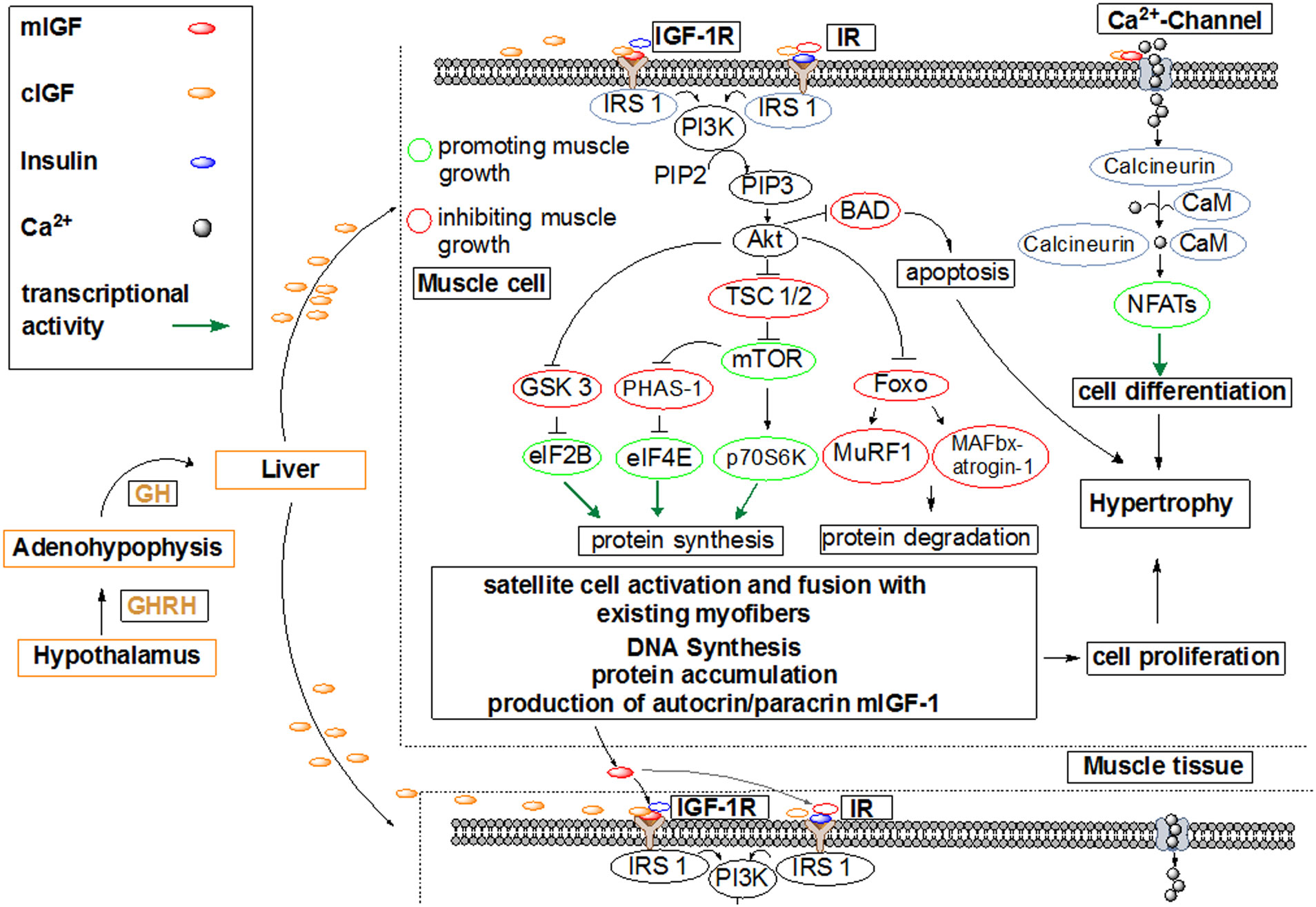
Velloso CP (2008) Regulation of muscle mass by growth hormone and IGF-I. Br J Pharmacol 154: 557–568. doi: 10.1038/bjp.2008.153
    [36] Enmark E, Gustafsson JA (1999) Oestrogen receptors - an overview. J Intern Med 246: 133–138. doi: 10.1046/j.1365-2796.1999.00545.x
    [37] Weigt C, Hertrampf T, Kluxen FM, et al. (2013) Molecular effects of ER alpha- and beta-selective agonists on regulation of energy homeostasis in obese female Wistar rats. Mol Cell Endocrinol 377: 147–158. doi: 10.1016/j.mce.2013.07.007
    [38] Lazovic G, Radivojevic U, Milosevic V, et al. (2007) Tibolone and osteoporosis. Arch Gynecol Obstet 276: 577–581. doi: 10.1007/s00404-007-0387-4
    [39] Narayanan R, Coss CC, Dalton JT (2018) Development of selective androgen receptor modulators (SARMs). Mol Cell Endocrinol 465: 134–142. doi: 10.1016/j.mce.2017.06.013
    [40] Gao WQ, Dalton JT (2007) Expanding the therapeutic use of androgens via selective androgen receptor modulators (SARMs). Drug Discovery Today 12: 241–248. doi: 10.1016/j.drudis.2007.01.003
    [41] Choo JJ, Horan MA, Little RA, et al. (1992) Anabolic effects of clenbuterol on skeletal muscle are mediated by beta 2-adrenoceptor activation. Am J Physiol 263: E50–56.
    [42] Moore N, Pegg G, Sillence M (1994) Anabolic effects of the beta2-andrenoceptor agonist salmeterol are dependent on route of administration. Am J Physiol 267: E475–E484.
    [43] Barbosa J, Cruz C, Martins J, et al. (2005) Food poisoning by clenbuterol in Portugal. Food Addit Contam 22: 563–566. doi: 10.1080/02652030500135102
    [44] Brambilla G, Cenci T, Franconi F, et al. (2000) Clinical and pharmacological profile in a clenbuterol epidemic poisoning of contaminated beef meat in Italy. Toxicol Lett 114: 47–53. doi: 10.1016/S0378-4274(99)00270-2
    [45] Sporano V, Grasso L, Esposito M, et al. (1998) Clenbuterol residues in non-liver containing meat as a cause of collective food poisoning. Vet Hum Toxicol 40: 141–143.
    [46] Brambilla G, Loizzo A, Fontana L, et al. (1997) Food poisoning following consumption of clenbuterol-treated veal in Italy. JAMA, J Am Med Assoc 278: 635.
    [47] Pulce C, Lamaison D, Keck G, et al. (1991) Collective human food poisonings by clenbuterol residues in veal liver. Vet Hum Toxicol 33: 480–481.
    [48] Salleras L, Dominguez A, Mata E, et al. (1995) Epidemiologic study of an outbreak of clenbuterol poisoning in Catalonia, Spain. Public Health Rep 110: 338–342.
    [49] Martinez-Navarro JF (1990) Food poisoning related to consumption of illicit beta-agonist in liver. Lancet 336: 1311.
    [50] Parr MK, Blokland MH, Liebetrau F, et al. (2017) Distinction of clenbuterol intake from drug or contaminated food of animal origin in a controlled administration trial - the potential of enantiomeric separation for doping control analysis. Food Addit Contam Part A Chem Anal Control Expo Risk Assess 34: 525–535. doi: 10.1080/19440049.2016.1242169
    [51] Parr MK, Opfermann G, Schanzer W (2009) Analytical methods for the detection of clenbuterol. Bioanalysis 1: 437–450. doi: 10.4155/bio.09.29
    [52] 
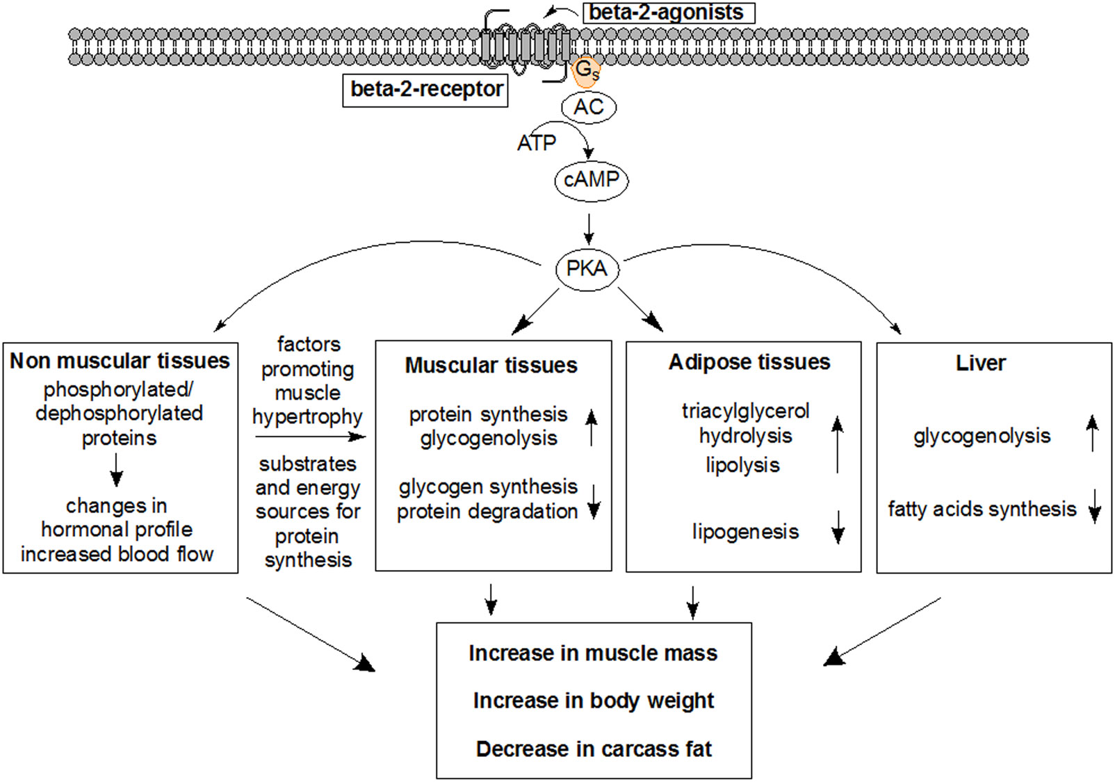
Mersmann HJ (1998) Overview of the effects of beta-adrenergic receptor agonists on animal growth including mechanisms of action. J Anim Sci 76: 160–172. doi: 10.2527/1998.761160x
    [53] World Anti-Doping Agency (2017) The 2018 Prohibited List. World Anti-Doping Agency.
    [54] Serra C, Bhasin S, Tangherlini F, et al. (2011) The role of GH and IGF-I in mediating anabolic effects of testosterone on androgen-responsive muscle. Endocrinology 152: 193–206. doi: 10.1210/en.2010-0802
    [55] Rommel C, Bodine SC, Clarke BA, et al. (2001) Mediation of IGF-1-induced skeletal myotube hypertrophy by PI(3)K/Akt/mTOR and PI(3)K/Akt/GSK3 pathways. Nat Cell Biol 3: 1009–1013. doi: 10.1038/ncb1101-1009
    [56] Bolster DR, Jefferson LS, Kimball SR (2004) Regulation of protein synthesis associated with skeletal muscle hypertrophy by insulin-, amino acid- and exercise-induced signalling. Proc Nutr Soc 63: 351–356. doi: 10.1079/PNS2004355
    [57] Holecek M (2017) Beta-hydroxy-beta-methylbutyrate supplementation and skeletal muscle in healthy and muscle-wasting conditions. J Cachexia Sarcopenia Muscle 8: 529–541. doi: 10.1002/jcsm.12208
    [58] Thomas M, Langley B, Berry C, et al. (2000) Myostatin, a negative regulator of muscle growth, functions by inhibiting myoblast proliferation. J Biol Chem 275: 40235–40243. doi: 10.1074/jbc.M004356200
    [59] Schuelke M, Wagner KR, Stolz LE, et al. (2004) Myostatin mutation associated with gross muscle hypertrophy in a child. N Engl J Med 350: 2682–2688. doi: 10.1056/NEJMoa040933
    [60] 
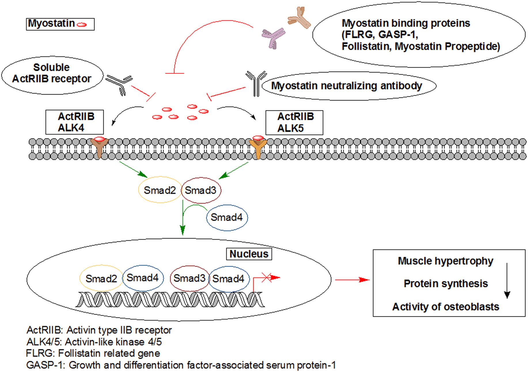
McPherron AC, Lawler AM, Lee SJ (1997) Regulation of skeletal muscle mass in mice by a new TGF-beta superfamily member. Nature 387: 83–90. doi: 10.1038/387083a0
    [61] Rı́os R, Carneiro I, Arce VM, et al. (2002) Myostatin is an inhibitor of myogenic differentiation. Am J Physiol Cell Physiol 282: C993–C999.
    [62] Sharma M, Langley B, Bass J, et al. (2001) Myostatin in muscle growth and repair. Exerc Sport Sci Rev 29: 155–158. doi: 10.1097/00003677-200110000-00004
    [63] Joulia-Ekaza D, Cabello G (2007) The myostatin gene: physiology and pharmacological relevance. Curr Opin Pharmacol 7: 310–315. doi: 10.1016/j.coph.2006.11.011
    [64] Elliott B, Renshaw D, Getting S, et al. (2012) The central role of myostatin in skeletal muscle and whole body homeostasis. Acta Physiol 205: 324–340. doi: 10.1111/j.1748-1716.2012.02423.x
    [65] Gonzalez-Cadavid NF, Taylor WE, Yarasheski K, et al. (1998) Organization of the human myostatin gene and expression in healthy men and HIV-infected men with muscle wasting. Proc Natl Acad Sci USA 95: 14938–14943. doi: 10.1073/pnas.95.25.14938
    [66] Pearen MA, Ryall JG, Maxwell MA, et al. (2006) The orphan nuclear receptor, NOR-1, is a target of beta-adrenergic signaling in skeletal muscle. Endocrinology 147: 5217–5227. doi: 10.1210/en.2006-0447
    [67] Ma K, Mallidis C, Bhasin S, et al. (2003) Glucocorticoid-induced skeletal muscle atrophy is associated with upregulation of myostatin gene expression. Am J Physiol Endocrinol Metab 285: E363–E371. doi: 10.1152/ajpendo.00487.2002
    [68] Chen PR, Lee K (2016) INVITED REVIEW: Inhibitors of myostatin as methods of enhancing muscle growth and development. J Anim Sci 94: 3125–3134. doi: 10.2527/jas.2016-0532
    [69] Dschietzig TB (2014) Myostatin - From the Mighty Mouse to cardiovascular disease and cachexia. Clin Chim Acta 433: 216–224. doi: 10.1016/j.cca.2014.03.021
    [70] Kung T, Springer J, Doehner W, et al. (2010) Novel treatment approaches to cachexia and sarcopenia: highlights from the 5th Cachexia Conference. Expert Opin Investig Drugs 19: 579–585. doi: 10.1517/13543781003724690
    [71] Rodgers BD, Garikipati DK (2008) Clinical, agricultural, and evolutionary biology of myostatin: a comparative review. Endocr Rev 29: 513–534. doi: 10.1210/er.2008-0003
    [72] Marchitelli C, Savarese MC, Crisa A, et al. (2003) Double muscling in Marchigiana beef breed is caused by a stop codon in the third exon of myostatin gene. Mammalian Genome 14: 392–395. doi: 10.1007/s00335-002-2176-5
    [73] Bellinge RH, Liberles DA, Iaschi SP, et al. (2005) Myostatin and its implications on animal breeding: a review. Anim Genet 36: 1–6. doi: 10.1111/j.1365-2052.2004.01229.x
    [74] Arnold H, Della-Fera M, Baile C (2001) Review of myostatin history, physiology and applications. Int Arch Biosci 1: 1014–1022.
    [75] Lee YS, Lehar A, Sebald S, et al. (2015) Muscle hypertrophy induced by myostatin inhibition accelerates degeneration in dysferlinopathy. Hum Mol Genet 24: 5711–5719. doi: 10.1093/hmg/ddv288
    [76] Bhasin S, Storer TW (2009) Anabolic applications of androgens for functional limitations associated with aging and chronic illness. Front Horm Res 37: 163–182.
    [77] Dobs AS, Boccia RV, Croot CC, et al. (2013) Effects of enobosarm on muscle wasting and physical function in patients with cancer: a double-blind, randomised controlled phase 2 trial. Lancet Oncol 14: 335–345. doi: 10.1016/S1470-2045(13)70055-X
    [78] Dillon EL, Durham WJ, Urban RJ, et al. (2010) Hormone treatment and muscle anabolism during aging: androgens. Clin Nutr 29: 697–700. doi: 10.1016/j.clnu.2010.03.010
    [79] Madeddu C, Maccio A, Mantovani G (2012) Multitargeted treatment of cancer cachexia. Crit Rev Oncog 17: 305–314. doi: 10.1615/CritRevOncog.v17.i3.80
    [80] Ebner N, Springer J, Kalantar-Zadeh K, et al. (2013) Mechanism and novel therapeutic approaches to wasting in chronic disease. Maturitas 75: 199–206. doi: 10.1016/j.maturitas.2013.03.014
    [81] Jasuja R, LeBrasseur NK (2014) Regenerating skeletal muscle in the face of aging and disease. Am J Phys Med Rehabil 93: S88–96. doi: 10.1097/PHM.0000000000000118
    [82] Madeddu C, Mantovani G, Gramignano G, et al. (2015) Advances in pharmacologic strategies for cancer cachexia. Expert Opin Pharmacother 16: 2163–2177. doi: 10.1517/14656566.2015.1079621
    [83] Srinath R, Dobs A (2014) Enobosarm (GTx-024, S-22): a potential treatment for cachexia. Future Oncol 10: 187–194. doi: 10.2217/fon.13.273
    [84] Forbes JM, Cooper ME (2013) Mechanisms of diabetic complications. Physiol Rev 93: 137-188. doi: 10.1152/physrev.00045.2011
    [85] Abdul-Ghani MA, DeFronzo RA (2010) Pathogenesis of insulin resistance in skeletal muscle. J Biomed Biotechnol 2010: 476279.
    [86] Heinlein CA, Chang C (2002) Androgen receptor (AR) coregulatros: An overview. Endocr Rev 23: 175–200. doi: 10.1210/edrv.23.2.0460
    [87] Hengevoss J, Piechotta M, Muller D, et al. (2015) Combined effects of androgen anabolic steroids and physical activity on the hypothalamic-pituitary-gonadal axis. J Steroid Biochem Mol Biol 150: 86–96. doi: 10.1016/j.jsbmb.2015.03.003
    [88] Murthy KS, Zhou H, Grider JR, et al. (2003) Inhibition of sustained smooth muscle contraction byPKA and PKG preferentially mediated by phosphorylation of RhoA. Am J Physiol Gastrointest Liver Physiol 284: G1006–1016.
    [89] Mahabadi V, Amory JK, Swerdloff RS, et al. (2009) Combined transdermal testosterone gel and the progestin nestorone suppresses serum gonadotropins in men. J Clin Endocrinol Metab 94: 2313–2320. doi: 10.1210/jc.2008-2604
    [90] Bonsall RW, Rees HD, Michael RP (1985) The distribution, nuclear uptake and metabolism of [3H]dihydrotestosterone in the brain, pituitary gland and genital tract of the male rhesus monkey. J Steroid Biochem 23: 389–398. doi: 10.1016/0022-4731(85)90184-0
    [91] Bonsall RW, Rees HD, Michael RP (1983) Characterization by high performance liquid chromatography of nuclear metabolites of testosterone in the brains of male rhesus monkeys. Life Sci 33: 655–663. doi: 10.1016/0024-3205(83)90254-0
    [92] Tilbrook AJ, Clarke IJ (2001) Negative feedback regulation of the secretion and actions of gonadotropin-releasing hormone in males. Biol Reprod 64: 735–742. doi: 10.1095/biolreprod64.3.735
    [93] Alen M, Reinila M, Vihko R (1985) Response of serum hormones to androgen administration in power athletes. Med Sci Sports Exerc 17: 354–359.
    [94] Smith CL, O'Malley BW (2004) Coregulator function: a key to understanding tissue specificity of selective receptor modulators. Endocr Rev 25: 45–71. doi: 10.1210/er.2003-0023
    [95] McEwan IJ (2013) Androgen receptor modulators: a marriage of chemistry and biology. Future Med Chem 5: 1109–1120. doi: 10.4155/fmc.13.69
    [96] Narayanan R, Coss CC, Yepuru M, et al. (2008) Steroidal androgens and nonsteroidal, tissue-selective androgen receptor modulator, S-22, regulate androgen receptor function through distinct genomic and nongenomic signaling pathways. Mol Endocrinol 22: 2448–2465. doi: 10.1210/me.2008-0160
    [97] Skelton DA, Phillips SK, Bruce SA, et al. (1999) Hormone replacement therapy increases isometric muscle strength of adductor pollicis in post-menopausal women. Clin Sci 96: 357–364. doi: 10.1042/cs0960357
    [98] Heikkinen J, Kyllonen E, Kurttila-Matero E, et al. (1997) HRT and exercise: effects on bone density, muscle strength and lipid metabolism. A placebo controlled 2-year prospective trial on two estrogen-progestin regimens in healthy postmenopausal women. Maturitas 26: 139–149.
    [99] Glenmark B, Nilsson M, Gao H, et al. (2004) Difference in skeletal muscle function in males vs. females: role of estrogen receptor-beta. Am J Physiol Endocrinol Metab 287: E1125–1131. doi: 10.1152/ajpendo.00098.2004
    [100] Velders M, Schleipen B, Fritzemeier KH, et al. (2012) Selective estrogen receptor-beta activation stimulates skeletal muscle growth and regeneration. FASEB J 26: 1909–1920. doi: 10.1096/fj.11-194779
    [101] Harris HA, Albert LM, Leathurby Y, et al. (2003) Evaluation of an estrogen receptor-beta agonist in animal models of human disease. Endocrinology 144: 4241–4249. doi: 10.1210/en.2003-0550
    [102] Martin C, Ross M, Chapman KE, et al. (2004) CYP7B generates a selective estrogen receptor beta agonist in human prostate. J Clin Endocrinol Metab 89: 2928–2935. doi: 10.1210/jc.2003-031847
    [103] Harris HA, Bruner-Tran KL, Zhang X, et al. (2005) A selective estrogen receptor-beta agonist causes lesion regression in an experimentally induced model of endometriosis. Hum Reprod 20: 936–941. doi: 10.1093/humrep/deh711
    [104] Norman BH, Dodge JA, Richardson TI, et al. (2006) Benzopyrans are selective estrogen receptor beta agonists with novel activity in models of benign prostatic hyperplasia. J Med Chem 49: 6155–6157. doi: 10.1021/jm060491j
    [105] Mersereau JE, Levy N, Staub RE, et al. (2008) Liquiritigenin is a plant-derived highly selective estrogen receptor beta agonist. Mol Cell Endocrinol 283: 49–57. doi: 10.1016/j.mce.2007.11.020
    [106] Piu F, Cheevers C, Hyldtoft L, et al. (2008) Broad modulation of neuropathic pain states by a selective estrogen receptor beta agonist. Eur J Pharmacol 590: 423–429. doi: 10.1016/j.ejphar.2008.05.015
    [107] Stovall DW, Pinkerton JV (2009) MF-101, an estrogen receptor beta agonist for the treatment of vasomotor symptoms in peri- and postmenopausal women. Curr Opin Investig Drugs 10: 365–371.
    [108] Roman-Blas JA, Castaneda S, Cutolo M, et al. (2010) Efficacy and safety of a selective estrogen receptor beta agonist, ERB-041, in patients with rheumatoid arthritis: a 12-week, randomized, placebo-controlled, phase II study. Arthritis Care Res 62: 1588–1593. doi: 10.1002/acr.20275
    [109] Robb EL, Stuart JA (2011) Resveratrol interacts with estrogen receptor-beta to inhibit cell replicative growth and enhance stress resistance by upregulating mitochondrial superoxide dismutase. Free Radic Biol Med 50: 821–831. doi: 10.1016/j.freeradbiomed.2010.12.038
    [110] Tagliaferri MA, Tagliaferri MC, Creasman JM, et al. (2016) A Selective Estrogen Receptor Beta Agonist for the Treatment of Hot Flushes: Phase 2 Clinical Trial. J Altern Complement Med 22: 722–728.
    [111] Leitman DC, Christians U (2012) MF101: a multi-component botanical selective estrogen receptor beta modulator for the treatment of menopausal vasomotor symptoms. Expert Opin Investig Drugs 21: 1031–1042. doi: 10.1517/13543784.2012.685652
    [112] Jackson RL, Greiwe JS, Schwen RJ (2011) Emerging evidence of the health benefits of S-equol, an estrogen receptor beta agonist. Nutr Rev 69: 432–448. doi: 10.1111/j.1753-4887.2011.00400.x
    [113] Weiser MJ, Wu TJ, Handa RJ (2009) Estrogen receptor-beta agonist diarylpropionitrile: biological activities of R- and S-enantiomers on behavior and hormonal response to stress. Endocrinology 150: 1817–1825. doi: 10.1210/en.2008-1355
    [114] Amer DA, Kretzschmar G, Muller N, et al. (2010) Activation of transgenic estrogen receptor-beta by selected phytoestrogens in a stably transduced rat serotonergic cell line. J Steroid Biochem Mol Biol 120: 208–217. doi: 10.1016/j.jsbmb.2010.04.018
    [115] Moutsatsou P (2007) The spectrum of phytoestrogens in nature: our knowledge is expanding. Hormones 6: 173–193.
    [116] Arias-Loza PA, Hu K, Dienesch C, et al. (2007) Both estrogen receptor subtypes, alpha and beta, attenuate cardiovascular remodeling in aldosterone salt-treated rats. Hypertension 50: 432–438. doi: 10.1161/HYPERTENSIONAHA.106.084798
    [117] Sun J, Baudry J, Katzenellenbogen JA, et al. (2003) Molecular basis for the subtype discrimination of the estrogen receptor-beta-selective ligand, diarylpropionitrile. Mol Endocrinol 17: 247–258. doi: 10.1210/me.2002-0341
    [118] Escande A, Pillon A, Servant N, et al. (2006) Evaluation of ligand selectivity using reporter cell lines stably expressing estrogen receptor alpha or beta. Biochem Pharmacol 71: 1459–1469. doi: 10.1016/j.bcp.2006.02.002
    [119] Ogawa M, Kitano T, Kawata N, et al. (2017) Daidzein down-regulates ubiquitin-specific protease 19 expression through estrogen receptor beta and increases skeletal muscle mass in young female mice. J Nutr Biochem 49: 63–70. doi: 10.1016/j.jnutbio.2017.07.017
    [120] Choi SY, Ha TY, Ahn JY, et al. (2008) Estrogenic activities of isoflavones and flavones and their structure-activity relationships. Planta Med 74: 25–32. doi: 10.1055/s-2007-993760
    [121] Zierau O, Kolba S, Olff S, et al. (2006) Analysis of the promoter-specific estrogenic potency of the phytoestrogens genistein, daidzein and coumestrol. Planta Med 72: 184–186. doi: 10.1055/s-2005-873182
    [122] Parr MK, Botre F, Nass A, et al. (2015) Ecdysteroids: A novel class of anabolic agents? Biol Sport 32: 169–173.
    [123] Kohara A, Machida M, Setoguchi Y, et al. (2017) Enzymatically modified isoquercitrin supplementation intensifies plantaris muscle fiber hypertrophy in functionally overloaded mice. J Int Soc Sports Nutr 14: 32. doi: 10.1186/s12970-017-0190-y
    [124] Foryst-Ludwig A, Clemenz M, Hohmann S, et al. (2008) Metabolic actions of estrogen receptor beta (ERbeta) are mediated by a negative cross-talk with PPARgamma. PLoS Genet 4: e1000108. doi: 10.1371/journal.pgen.1000108
    [125] Semple RK, Chatterjee VK, O'Rahilly S (2006) PPAR gamma and human metabolic disease. J Clin Invest 116: 581–589. doi: 10.1172/JCI28003
    [126] Glass DJ (2005) Skeletal muscle hypertrophy and atrophy signaling pathways. Int J Biochem Cell Biol 37: 1974–1984. doi: 10.1016/j.biocel.2005.04.018
    [127] Bodine SC, Stitt TN, Gonzalez M, et al. (2001) Akt/mTOR pathway is a crucial regulator of skeletal muscle hypertrophy and can prevent muscle atrophy in vivo. Nat Cell Biol 3: 1014–1019. doi: 10.1038/ncb1101-1014
    [128] Wang M, Wang Y, Weil B, et al. (2009) Estrogen receptor beta mediates increased activation of PI3K/Akt signaling and improved myocardial function in female hearts following acute ischemia. Am J Physiol Regul Integr Comp Physiol 296: R972–978. doi: 10.1152/ajpregu.00045.2009
    [129] Stitt TN, Drujan D, Clarke BA, et al. (2004) The IGF-1/PI3K/Akt pathway prevents expression of muscle atrophy-induced ubiquitin ligases by inhibiting FOXO transcription factors. Mol Cell 14: 395–403. doi: 10.1016/S1097-2765(04)00211-4
    [130] Guttdrige D (2004) Signaling pathways weigh in on decisions to make or break skeletal muscle. Curr Opin Clin Nutr Metab Care 7: 443–450. doi: 10.1097/01.mco.0000134364.61406.26
    [131] Nader GA (2005) Molecular determinants of skeletal muscle mass: getting the "AKT" together. Int J Biochem Cell Biol 37: 1985–1996. doi: 10.1016/j.biocel.2005.02.026
    [132] Glass DJ (2010) Signaling pathways perturbing muscle mass. Curr Opin Clin Nutr Metab Care 13: 225–229. doi: 10.1097/MCO.0b013e32833862df
    [133] Song YH, Godard M, Li Y, et al. (2005) Insulin-like growth factor I-mediated skeletal muscle hypertrophy is characterized by increased mTOR-p70S6K signaling without increased Akt phosphorylation. J Investig Med 53: 135–142. doi: 10.2310/6650.2005.00309
    [134] Glass DJ (2003) Signalling pathways that mediate skeletal muscle hypertrophy and atrophy. Nat Cell Biol 5: 87–90. doi: 10.1038/ncb0203-87
    [135] Schiaffino S, Mammucari C (2011) Regulation of skeletal muscle growth by the IGF1-Akt/PKB pathway: insights from genetic models. Skelet Muscle 1: 4. doi: 10.1186/2044-5040-1-4
    [136] Lux MP, Fasching PA, Schrauder MG, et al. (2016) The PI3K Pathway: Background and Treatment Approaches. Breast Care 11: 398–404. doi: 10.1159/000453133
    [137] MacLennan P, Edwards R (1989) Effects of clenbuterol and propanolol on muscle mass. Biochem J 264: 573–579. doi: 10.1042/bj2640573
    [138] Schmidt P, Holsboer F, Spengler D (2001) β2-Adrenergic Receptors Potentiate Glucocorticoid Receptor Transactivation via G Proteinβγ-Subunits and the Phosphoinositide 3-Kinase Pathway. Mol Endocrinol 15: 553–564.
    [139] Murga C, Laguinge L, Wetzker R, et al. (1998) Activation of Akt/Protein Kinase B by G Protein-coupled Receptors A ROLE FOR α AND βγ SUBUNITS OF HETEROTRIMERIC G PROTEINS ACTING THROUGH PHOSPHATIDYLINOSITOL-3-OH KINASEγ. J Biol Chem 273: 19080–19085. doi: 10.1074/jbc.273.30.19080
    [140] Huang P, Li Y, Lv Z, et al. (2017) Comprehensive attenuation of IL-25-induced airway hyperresponsiveness, inflammation and remodelling by the PI3K inhibitor LY294002. Respirology 22: 78–85.
    [141] Welle S, Burgess K, Mehta S (2009) Stimulation of skeletal muscle myofibrillar protein synthesis, p70 S6 kinase phosphorylation, and ribosomal protein S6 phosphorylation by inhibition of myostatin in mature mice. Am J Physiol Endocrinol Metab 296: E567–572. doi: 10.1152/ajpendo.90862.2008
    [142] Jefferies HB, Fumagalli S, Dennis PB, et al. (1997) Rapamycin suppresses 5' TOP mRNA translation through inhibition of p70 s6k. EMBO J 16: 3693–3704. doi: 10.1093/emboj/16.12.3693
    [143] Beretta L, Gingras AC, Svitkin YV, et al. (1996) Rapamycin blocks the phosphorylation of 4E-BP1 and inhibits cap-dependent initiation of translation. EMBO J 15: 658–664.
    [144] Sneddon AA, Delday MI, Steven J, et al. (2001) Elevated IGF-II mRNA and phosphorylation of 4E-BP1 and p70S6k in muscle showing clenbuterol-induced anabolism. Am J Physiol Endocrinol Metab 281: E676–E682. doi: 10.1152/ajpendo.2001.281.4.E676
    [145] Bodine SC, Latres E, Baumhueter S, et al. (2001) Identification of ubiquitin ligases required for skeletal muscle atrophy. Science 294: 1704–1708. doi: 10.1126/science.1065874
    [146] Kline WO, Panaro FJ, Yang H, et al. (2007) Rapamycin inhibits the growth and muscle-sparing effects of clenbuterol. J Appl Physiol (1985) 102: 740–747. doi: 10.1152/japplphysiol.00873.2006
    [147] Okumura S, Fujita T, Cai W, et al. (2014) Epac1-dependent phospholamban phosphorylation mediates the cardiac response to stresses. J Clin Invest 124: 2785–2801. doi: 10.1172/JCI64784
    [148] Ohnuki Y, Umeki D, Mototani Y, et al. (2014) Role of cyclic AMP sensor Epac1 in masseter muscle hypertrophy and myosin heavy chain transition induced by beta2-adrenoceptor stimulation. J Physiol 592: 5461–5475. doi: 10.1113/jphysiol.2014.282996
    [149] Ohnuki Y, Umeki D, Mototani Y, et al. (2016) Role of phosphodiesterase 4 expression in the Epac1 signaling-dependent skeletal muscle hypertrophic action of clenbuterol. Physiol Rep 4.
    [150] Burnett DD, Paulk CB, Tokach MD, et al. (2016) Effects of Added Zinc on Skeletal Muscle Morphometrics and Gene Expression of Finishing Pigs Fed Ractopamine-HCL. Anim Biotechnol 27: 17–29. doi: 10.1080/10495398.2015.1069301
    [151] Py G, Ramonatxo C, Sirvent P, et al. (2015) Chronic clenbuterol treatment compromises force production without directly altering skeletal muscle contractile machinery. J Physiol 593: 2071–2084. doi: 10.1113/jphysiol.2014.287060
    [152] Rena G, Guo S, Cichy SC, et al. (1999) Phosphorylation of the transcription factor forkhead family member FKHR by protein kinase B. J Biol Chem 274: 17179–17183. doi: 10.1074/jbc.274.24.17179
    [153] Biggs WH, 3rd, Meisenhelder J, Hunter T, et al. (1999) Protein kinase B/Akt-mediated phosphorylation promotes nuclear exclusion of the winged helix transcription factor FKHR1. Proc Natl Acad Sci U S A 96: 7421–7426. doi: 10.1073/pnas.96.13.7421
    [154] Umeki D, Ohnuki Y, Mototani Y, et al. (2015) Protective Effects of Clenbuterol against Dexamethasone-Induced Masseter Muscle Atrophy and Myosin Heavy Chain Transition. PLoS One 10: e0128263. doi: 10.1371/journal.pone.0128263
    [155] de Palma L, Marinelli M, Pavan M, et al. (2008) Ubiquitin ligases MuRF1 and MAFbx in human skeletal muscle atrophy. Joint Bone Spine 75: 53–57. doi: 10.1016/j.jbspin.2007.04.019
    [156] Gomez-SanMiguel AB, Gomez-Moreira C, Nieto-Bona MP, et al. (2016) Formoterol decreases muscle wasting as well as inflammation in the rat model of rheumatoid arthritis. Am J Physiol Endocrinol Metab 310: E925–937. doi: 10.1152/ajpendo.00503.2015
    [157] Jesinkey SR, Korrapati MC, Rasbach KA, et al. (2014) Atomoxetine prevents dexamethasone-induced skeletal muscle atrophy in mice. J Pharmacol Exp Ther 351: 663–673. doi: 10.1124/jpet.114.217380
    [158] Yang YT, McElligott MA (1989) Multiple actions of beta-adrenergic agonists on skeletal muscle and adipose tissue. Biochem J 261: 1–10. doi: 10.1042/bj2610001
    [159] Peterla TA, Scanes CG (1990) Effect of beta-adrenergic agonists on lipolysis and lipogenesis by porcine adipose tissue in vitro. J Anim Sci 68: 1024–1029. doi: 10.2527/1990.6841024x
    [160] Mayr B, Montminy M (2001) Transcriptional regulation by the phosphorylation-dependent factor CREB. Nat Rev Mol Cell Biol 2: 599–609.
    [161] Pearen MA, Myers SA, Raichur S, et al. (2008) The orphan nuclear receptor, NOR-1, a target of beta-adrenergic signaling, regulates gene expression that controls oxidative metabolism in skeletal muscle. Endocrinology 149: 2853–2865. doi: 10.1210/en.2007-1202
    [162] Martinez JA, Portillo MP, Larralde J (1991) Anabolic actions of a mixed beta-adrenergic agonist on nitrogen retention and protein turnover. Horm Metab Res 23: 590–593. doi: 10.1055/s-2007-1003762
    [163] Watkins LE, Jones DJ, Mowrey DH, et al. (1990) The Effect of Various Levels of Ractopamine Hydrochloride on the Performance and Carcass Characteristics of Finishing Swine. J Anim Sci 68: 3588–3595. doi: 10.2527/1990.68113588x
    [164] Crome PK, McKeith FK, Carr TR, et al. (1996) Effect of ractopamine on growth performance, carcass composition, and cutting yields of pigs slaughtered at 107 and 125 kilograms. J Anim Sci 74: 709–716. doi: 10.2527/1996.744709x
    [165] Adams GR, Haddad F (1996) The relationships among IGF-1, DNA content, and protein accumulation during skeletal muscle hypertrophy. J Applied Physiol 81: 2509–2516. doi: 10.1152/jappl.1996.81.6.2509
    [166] Adams GR (2002) Invited Review: Autocrine/paracrine IGF-I and skeletal muscle adaptation. J Appl Physiol 93: 1159–1167. doi: 10.1152/japplphysiol.01264.2001
    [167] Grounds MD (2002) Reasons for the degeneration of ageing skeletal muscle: a central role for IGF-1 signalling. Biogerontology 3: 19–24. doi: 10.1023/A:1015234709314
    [168] Kicman AT, Miell JP, Teale JD, et al. (1997) Serum IGF-I and IGF binding proteins 2 and 3 as potential markers of doping with human GH. Clin Endocrinol 47: 43–50. doi: 10.1046/j.1365-2265.1997.2111036.x
    [169] Bahl N, Stone G, McLean M, et al. (2018) Decorin, a growth hormone-regulated protein in humans. Eur J Endocrinol 178: 147–154. doi: 10.1530/EJE-17-0844
    [170] Kanzleiter T, Rath M, Gorgens SW, et al. (2014) The myokine decorin is regulated by contraction and involved in muscle hypertrophy. Biochem Biophys Res Commun 450: 1089–1094. doi: 10.1016/j.bbrc.2014.06.123
    [171] Musaro A, McCullagh K, Paul A, et al. (2001) Localized Igf-1 transgene expression sustains hypertrophy and regeneration in senescent skeletal muscle. Nat Genet 27: 195–200. doi: 10.1038/84839
    [172] Adams GR, McCue SA (1998) Localized infusion of IGF-I results in skeletal muscle hypertrophy in rats. J Appl Physiol 84: 1716–1722. doi: 10.1152/jappl.1998.84.5.1716
    [173] Yin HN, Chai JK, Yu YM, et al. (2009) Regulation of signaling pathways downstream of IGF-I/insulin by androgen in skeletal muscle of glucocorticoid-treated rats. J Trauma 66: 1083–1090. doi: 10.1097/TA.0b013e31817e7420
    [174] Jang YJ, Son HJ, Choi YM, et al. (2017) Apigenin enhances skeletal muscle hypertrophy and myoblast differentiation by regulating Prmt7. Oncotarget 8: 78300–78311.
    [175] Song YH, Li Y, Du J, et al. (2005) Muscle-specific expression of IGF-1 blocks angiotensin II-induced skeletal muscle wasting. J Clin Invest 115: 451–458. doi: 10.1172/JCI22324
    [176] LaVigne EK, Jones AK, Londono AS, et al. (2015) Muscle growth in young horses: Effects of age, cytokines, and growth factors. J Anim Sci 93: 5672–5680. doi: 10.2527/jas.2015-9634
    [177] Chin ER, Olson EN, Richardson JA, et al. (1998) A calcineurin-dependent transcriptional pathway controls skeletal muscle fiber type. Genes Dev 12: 2499–2509. doi: 10.1101/gad.12.16.2499
    [178] Delling U, Tureckova J, Lim HW, et al. (2000) A calcineurin-NFATc3-dependent pathway regulates skeletal muscle differentiation and slow myosin heavy-chain expression. Mol Cell Biol 20: 6600–6611. doi: 10.1128/MCB.20.17.6600-6611.2000
    [179] Semsarian C, Wu MJ, Ju YK, et al. (1999) Skeletal muscle hypertrophy is mediated by a Ca2+-dependent calcineurin signalling pathway. Nature 400: 576–581. doi: 10.1038/23054
    [180] Miyashita T, Takeishi Y, Takahashi H, et al. (2001) Role of calcineurin in insulin-like growth factor-1-induced hypertrophy of cultured adult rat ventricular myocytes. Jpn Circ J 65: 815–819. doi: 10.1253/jcj.65.815
    [181] Musaro A, McCullagh KJA, Naya FJ, et al. (1999) IGF-1 induces skeletal myocyte hypertrophy through calcineurin in association with GATA-2 and NF-ATc1. Nature 400: 581–585. doi: 10.1038/23060
    [182] Swoap SJ, Hunter RB, Stevenson EJ, et al. (2000) The calcineurin-NFAT pathway and muscle fiber-type gene expression. Am J Physiol Cell Physiol 279: C915–C924. doi: 10.1152/ajpcell.2000.279.4.C915
    [183] White TA, LeBrasseur NK (2014) Myostatin and sarcopenia: opportunities and challenges - a mini-review. Gerontology 60: 289–293. doi: 10.1159/000356740
    [184] Patel K, Amthor H (2005) The function of Myostatin and strategies of Myostatin bloackde - new hope for therapies aimed at promoting growth of skeletal muscle. Neuromuscular Disord 15: 117–126. doi: 10.1016/j.nmd.2004.10.018
    [185] Sartori R, Milan G, Patron M, et al. (2009) Smad2 and 3 transcription factors control muscle mass in adulthood. Am J Physiol Cell Physiol 296: C1248–1257. doi: 10.1152/ajpcell.00104.2009
    [186] Smith RC, Lin BK (2013) Moystatin inhibitors as therapies for muscle wasting associated with cancer and other disorders. Curr Opin Support Palliat Care 7: 352–360. doi: 10.1097/SPC.0000000000000013
    [187] Winbanks CE, Weeks KL, Thomson RE, et al. (2012) Follistatin-mediated skeletal muscle hypertrophy is regulated by Smad3 and mTOR independently of myostatin. J Cell Biol 197: 997–1008. doi: 10.1083/jcb.201109091
    [188] Winbanks CE, Chen JL, Qian H, et al. (2013) The bone morphogenetic protein axis is a positive regulator of skeletal muscle mass. J Cell Biol 203: 345–357. doi: 10.1083/jcb.201211134
    [189] Barbe C, Kalista S, Loumaye A, et al. (2015) Role of IGF-I in follistatin-induced skeletal muscle hypertrophy. Am J Physiol Endocrinol Metab 309: E557–567. doi: 10.1152/ajpendo.00098.2015
    [190] Wang Q, Guo T, Portas J, et al. (2015) A soluble activin receptor type IIB does not improve blood glucose in streptozotocin-treated mice. Int J Biol Sci 11: 199–208. doi: 10.7150/ijbs.10430
    [191] Barreiro E, Tajbakhsh S (2017) Epigenetic regulation of muscle development. J Muscle Res Cell Motil 38: 31–35. doi: 10.1007/s10974-017-9469-5
    [192] Grazioli E, Dimauro I, Mercatelli N, et al. (2017) Physical activity in the prevention of human diseases: role of epigenetic modifications. BMC Genomics 18: 802. doi: 10.1186/s12864-017-4193-5
    [193] Saccone V, Puri PL (2010) Epigenetic regulation of skeletal myogenesis. Organogenesis 6: 48–53. doi: 10.4161/org.6.1.11293
    [194] Sincennes MC, Brun CE, Rudnicki MA (2016) Concise Review: Epigenetic Regulation of Myogenesis in Health and Disease. Stem Cells Transl Med 5: 282–290. doi: 10.5966/sctm.2015-0266
    [195] Townley-Tilson WH, Callis TE, Wang D (2010) MicroRNAs 1, 133, and 206: critical factors of skeletal and cardiac muscle development, function, and disease. Int J Biochem Cell Biol 42: 1252–1255. doi: 10.1016/j.biocel.2009.03.002
    [196] Proctor CJ, Goljanek-Whysall K (2017) Using computer simulation models to investigate the most promising microRNAs to improve muscle regeneration during ageing. Sci Rep 7: 12314. doi: 10.1038/s41598-017-12538-6
    [197] Yu H, Lu Y, Li Z, et al. (2014) microRNA-133: expression, function and therapeutic potential in muscle diseases and cancer. Curr Drug Targets 15: 817–828. doi: 10.2174/1389450115666140627104151
  • Reader Comments
  • © 2018 the Author(s), licensee AIMS Press. This is an open access article distributed under the terms of the Creative Commons Attribution License (http://creativecommons.org/licenses/by/4.0)
通讯作者: 陈斌, bchen63@163.com
  • 1. 

    沈阳化工大学材料科学与工程学院 沈阳 110142

  1. 本站搜索
  2. 百度学术搜索
  3. 万方数据库搜索
  4. CNKI搜索

Metrics

Article views(12816) PDF downloads(2582) Cited by(6)

Figures and Tables

Figures(7)

Other Articles By Authors

/

DownLoad:  Full-Size Img  PowerPoint
Return
Return

Catalog