Effect of Gaussian filtered images on Mask RCNN in detection and segmentation of potholes in smart cities

Auwalu Saleh Mubarak; Zubaida Said Ameen; Fadi Al-Turjman; Auwalu Saleh Mubarak; Zubaida Said Ameen; Fadi Al-Turjman

doi:10.3934/mbe.2023013

Mathematical Biosciences and Engineering

2023, Volume 20, Issue 1: 283-295. doi: 10.3934/mbe.2023013

Previous Article Next Article

Research article Special Issues

Effect of Gaussian filtered images on Mask RCNN in detection and segmentation of potholes in smart cities

1.
Artificial Intelligence Engineering Dept., AI and Robotics Institute, Near East University, Mersin 10, Turkey
2.
Electrical Engineering Dept., Kano University of Science and Technology, Wudil, Kano, Nigeria
3.
Biochemistry Dept., Maitama Sule University, Kano, Nigeria
4.
Research Center for AI and IoT, Faculty of Engineering, University of Kyrenia, Kyrenia, Mersin 10, Turkey

Academic Editor: Byung-Gyu Kim

Received: 26 July 2022 Revised: 30 August 2022 Accepted: 09 September 2022 Published: 30 September 2022

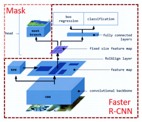
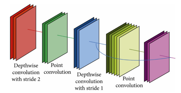
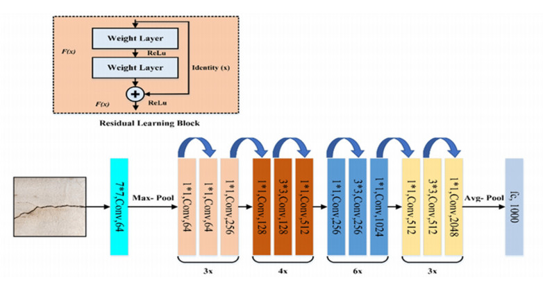
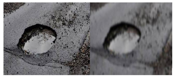
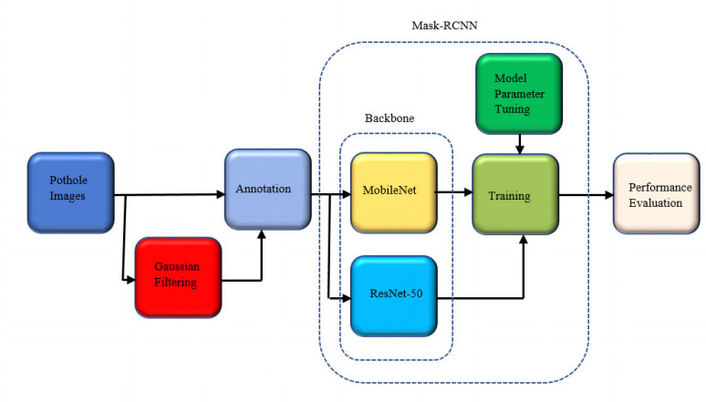
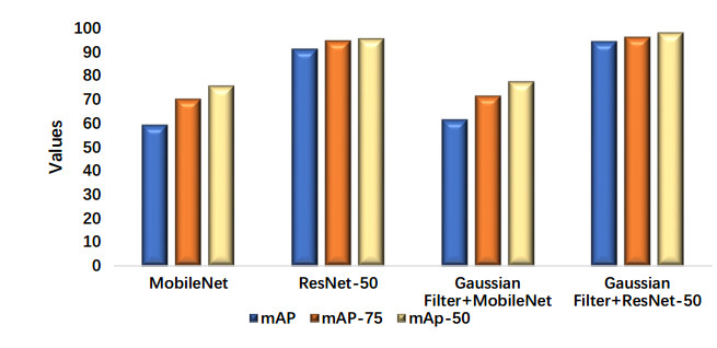
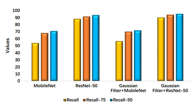
Accidents have contributed a lot to the loss of lives of motorists and serious damage to vehicles around the globe. Potholes are the major cause of these accidents. It is very important to build a model that will help in recognizing these potholes on vehicles. Several object detection models based on deep learning and computer vision were developed to detect these potholes. It is very important to develop a lightweight model with high accuracy and detection speed. In this study, we employed a Mask RCNN model with ResNet-50 and MobileNetv1 as the backbone to improve detection, and also compared the performance of the proposed Mask RCNN based on original training images and the images that were filtered using a Gaussian smoothing filter. It was observed that the ResNet trained on Gaussian filtered images outperformed all the employed models.

Keywords:

Citation: Auwalu Saleh Mubarak, Zubaida Said Ameen, Fadi Al-Turjman. Effect of Gaussian filtered images on Mask RCNN in detection and segmentation of potholes in smart cities[J]. Mathematical Biosciences and Engineering, 2023, 20(1): 283-295. doi: 10.3934/mbe.2023013

Related Papers:

[1]	Xingjia Li, Jinan Gu, Zedong Huang, Chen Ji, Shixi Tang . Hierarchical multiloop MPC scheme for robot manipulators with nonlinear disturbance observer. Mathematical Biosciences and Engineering, 2022, 19(12): 12601-12616. doi: 10.3934/mbe.2022588
[2]	Xingjia Li, Jinan Gu, Zedong Huang, Wenbo Wang, Jing Li . Optimal design of model predictive controller based on transient search optimization applied to robotic manipulators. Mathematical Biosciences and Engineering, 2022, 19(9): 9371-9387. doi: 10.3934/mbe.2022436
[3]	Van Dong Nguyen, Dinh Quoc Vo, Van Tu Duong, Huy Hung Nguyen, Tan Tien Nguyen . Reinforcement learning-based optimization of locomotion controller using multiple coupled CPG oscillators for elongated undulating fin propulsion. Mathematical Biosciences and Engineering, 2022, 19(1): 738-758. doi: 10.3934/mbe.2022033
[4]	Ruiping Yuan, Jiangtao Dou, Juntao Li, Wei Wang, Yingfan Jiang . Multi-robot task allocation in e-commerce RMFS based on deep reinforcement learning. Mathematical Biosciences and Engineering, 2023, 20(2): 1903-1918. doi: 10.3934/mbe.2023087
[5]	Xinyu Shao, Zhen Liu, Baoping Jiang . Sliding-mode controller synthesis of robotic manipulator based on a new modified reaching law. Mathematical Biosciences and Engineering, 2022, 19(6): 6362-6378. doi: 10.3934/mbe.2022298
[6]	Xinran Zhang, Yongde Zhang, Jianzhi Yang, Haiyan Du . A prostate seed implantation robot system based on human-computer interactions: Augmented reality and voice control. Mathematical Biosciences and Engineering, 2024, 21(5): 5947-5971. doi: 10.3934/mbe.2024262
[7]	Yongli Yan, Fucai Liu, Teng Ren, Li Ding . Nonlinear extended state observer based control for the teleoperation of robotic systems with flexible joints. Mathematical Biosciences and Engineering, 2024, 21(1): 1203-1227. doi: 10.3934/mbe.2024051
[8]	Juan Du, Jie Hou, Heyang Wang, Zhi Chen . Application of an improved whale optimization algorithm in time-optimal trajectory planning for manipulators. Mathematical Biosciences and Engineering, 2023, 20(9): 16304-16329. doi: 10.3934/mbe.2023728
[9]	Mubashir Ahmad, Saira, Omar Alfandi, Asad Masood Khattak, Syed Furqan Qadri, Iftikhar Ahmed Saeed, Salabat Khan, Bashir Hayat, Arshad Ahmad . Facial expression recognition using lightweight deep learning modeling. Mathematical Biosciences and Engineering, 2023, 20(5): 8208-8225. doi: 10.3934/mbe.2023357
[10]	Kun Zhai, Qiang Ren, Junli Wang, Chungang Yan . Byzantine-robust federated learning via credibility assessment on non-IID data. Mathematical Biosciences and Engineering, 2022, 19(2): 1659-1676. doi: 10.3934/mbe.2022078

Abstract

1. Introduction

Differential equations are used to describe dynamic evolutionary processes in natural sciences, engineering and technology. There are many mathematicians working to construct methods for computing exact solutions to differential equations: for example, the Bäcklund transformation method ^[1], the inverse scattering method ^[2], the Darboux transformation method ^[3], the Hirota bilinear method ^[4], the tanh-function method ^[5], the Homotopy analysis method ^[6], etc. In recent years, there have been many results in constructing exact solutions of partial differential equations with a finite number of integer-order derivatives, such as the conformable fractional derivative, the M-fractional derivative, the alternative fractional derivative, the local fractional derivative and the Caputo-Fabrizio fractional derivatives with exponential kernels.

In Tarasov's points, the above mentioned differential operators are not fractional, with exponential kernels that cannot be considered as fractional derivatives of non-integer orders ^[7]. Therefore, the method designed for differential operators with integer orders can be embedded in the above mentioned type of differential equations with derivative variants.

For the question of how to distinguish between differential equations with integer-order and with fractional order, Tarasov introduced the nonlocality principle to prove that the conformable fractional derivative with exponential kernels cannot be considered as fractional derivatives of non-integer orders ^[7]. The derivatives of integer orders are determined by properties of differentiable functions only in the infinitely small neighborhoods of the considered point but not nonlocal. In the sense of conformable derivatives, the fractional differential problems become differential problems with integer-order derivatives that may no longer properly describe the original fractional physical phenomena ^[8]. Many mathematicians have worked on improving the conformable derivative to make it have more complete properties or apply more; for examples, see ^[9,10,11,12].

There are many ways of find exact solutions of differential equations, but no single method can handle all types of solutions. The complex method ^[13,14,15] and its variants, such as the extended complex method ^[16], can be used to construct meromorphic solutions for certain partial differential equations. Several researchers have tried to apply the complex method to find exact solutions of some higher-order or higher-dimension partial differential equations; for examples, see ^[17,18]. The complex method will be used here because this kind of method can construct more types of solutions in the complex domain, such as elliptic function solutions, simply periodic function solutions and exponential function solutions. Also, this is a good attempt to solve differential equations with conformal derivatives by the complex method.

Shallow waters exhibit nonlinear phenomena in the propagation and transformation of waves. Nonlinear differential equations, such as the Huxley equation, describe spectral energy transfer for waves of finite amplitude in shallow waters above a flat seafloor ^[19,20]. Chaotic oscillations usually occur in nonlinear dynamical systems. These systems can be represented by the Huxley equation with nonlinear oscillations and external periodic excitation ^[21].

Although the sub-equation method, the Kudryashov method and the exp-function method have been applied to build exact solutions for the conformable Huxley equation ^[22] (see Eq (3.1)), we remain committed to finding abundant new exact solutions using the complex method. The new exact solutions may contribute to a much better understanding of the features of the solutions of the conformable Huxley equation.

2. Preliminaries

The basic definition and theorems of conformable derivatives ^[23] are as follows.

Definition 2.1. Let $g: (0, \infty) \rightarrow R$ be a function. For all $k > 0, \alpha \in (0, 1)$ , the CFD of $g$ for order $\alpha$ is defined by

$\begin{equation} T_{\alpha}(g(k)) = \lim _{\varepsilon \rightarrow 0} \frac{g\left(k+\varepsilon k^{1-\alpha}\right)-g(k)}{\varepsilon}. \end{equation}$

(2.1)

Lemma 2.1. For $\alpha \in (0, 1]$ , if a function $g: (0, +\infty) \rightarrow R$ is $\alpha$ -differentiable at $t_0 > 0$ , then $g$ is continuous at $t_0$ .

Lemma 2.2. Let $f$ and $g$ be $\alpha$ -differential at a point $t > 0$ , $\alpha \in (0, 1]$ .

$\begin{equation} \begin{split} T_{\alpha}(\alpha f+b g) & = a T_{\alpha}(f)+b T_{\alpha}(g), \mathit{\text{for all}}~~ a, b \in R , \\ T_{\alpha}\left(t^{p}\right) & = p t^{p-\alpha}, \mathit{\text{for all}}~~ p \in R, \\ T_{\alpha}(\lambda) & = 0, \mathit{\text{for all constant functions}}~~ f(t) = \lambda, \\ T_{\alpha}(f g) & = f T_{\alpha}(g)+g T_{\alpha}(f)~~ \mathit{\text{and}}\\ T_{\alpha}\left(\frac{f}{g}\right) & = \frac{g T_{\alpha}(f)-f T_{\alpha}(g)}{g^{2}}. \end{split} \end{equation}$

(2.2)

If $g$ is differentiable,

$\begin{equation} T_{\alpha}(g)(t) = t^{1-\alpha} \frac{d g}{d t}(t). \end{equation}$

(2.3)

Giving a nonlinear conformable partial differential equation with two independent variables,

$\begin{equation} P\left(\frac{\partial^{\alpha} u}{\partial t~ ^{\alpha}}, \frac{\partial u}{\partial x}, \frac{\partial^{2 \alpha} u}{\partial t^{2 \alpha}}, \frac{\partial^{2} u}{\partial x^{2}}, \cdots\right) = 0, 0 < \alpha \leq 1. \end{equation}$

(2.4)

Taking a traveling wave transformation $u(x, t) = w(z), z = x-c\frac{t~ ^{\alpha}}{\alpha}~~$ ( $c$ is the speed of wave), on Eq (2.4) with

$\begin{equation} \frac{\partial^{\alpha}}{\partial t~ ^{\alpha}} = -c \frac{\partial}{\partial \xi}, \frac{\partial^{2 \alpha}}{\partial t^{2 \alpha}} = c^{2} \frac{\partial^{2}}{\partial \xi^{2}}, \frac{\partial}{\partial x} = \frac{\partial}{\partial \xi}, \frac{\partial^{2}}{\partial x^{2}} = \frac{\partial^{2}}{\partial \xi^{2}}, \cdots, \end{equation}$

(2.5)

Eq (2.4) will be reduced to a nonlinear ordinary differential equation (ODE),

$\begin{equation} Q(w, w', w'', w''', \cdots) = 0. \end{equation}$

(2.6)

Weierstrass elliptic function ^[24] $\wp(z): = \wp(z, g_2, g_3)$ is a meromorphic function with two periods $2\omega_1, \; 2\omega_2$ and satisfies

$\begin{equation} (\wp'(z))^2 = 4 \wp(z)^3-g_2 \wp(z)-g_3, \end{equation}$

(2.7)

with the invariants $g_2 = 60s_4, \; g_3 = 140s_6$ and discriminant $\Delta(g_2, g_3)\neq 0.$

Furthermore, $\wp'(-z) = -\wp'(z)$ , $2\wp''(z) = 12\wp^2(z)-g_2, \wp'''(z) = 12\wp(z)\wp'(z), \cdots$ , any $k$ th derivatives of $\wp$ can be deduced by these identities, and $\wp$ has the Laurent series expansion $\wp(z) = \frac{1}{z^2}+\frac{g_2z^2}{20}+\frac{g_3z^4}{28}+O(|z|^6)$ , with the addition formula

$\begin{equation} \wp(z-z_0) = -\wp(z)-\wp(z_0)+\frac{1}{4}[\frac{\wp'(z)+\wp'(z_0)}{\wp(z)-\wp(z_0)}]^2. \end{equation}$

(2.8)

The basic related definitions and lemmas of the complex method ^[13] are as follows.

Given a nonlinear ODE

$\begin{equation} P(w, w', \cdots, w^{(m)}) = 0, \end{equation}$

(2.9)

$P$ is a polynomial in $w(z)$ and its derivatives with constant coefficients.

We assume that the Laurent series expansion of meromorphic solutions of Eq (2.9) are in the form of

$\begin{equation} w(z) = \sum\limits_{k = -q}^{\infty}c_{k}(z-z_0)^k\; (q > 0). \end{equation}$

(2.10)

Definition 2.2. If there are exactly $p$ distinct formal meromorphic Laurent series

$\begin{equation} w(z) = \sum\limits_{k = -q}^{\infty}c_{k}z^{k} \end{equation}$

(2.11)

satisfying Eq (2.9), we say Eq (2.9) satisfies the $\langle p, q \rangle$ condition. If only determine $p$ distinct principal parts $\sum_{k = -q}^{-1}c_{k}z^{k}$ , we say Eq (2.9) satisfies the weak $\langle p, q \rangle$ condition.

Eremenko ^[25] defined that a meromorphic function $f(z)$ belongs to the class $W$ if $f(z)$ is an elliptic function, a rational function of $e^{\alpha z}(\alpha\in\mathbb{C})$ or a rational function of $z$ .

Lemma 2.3. (^[13,15]) Suppose that an equation

$\begin{equation} P(w, w', \cdots, w^{(m)}) = bw^n \end{equation}$

(2.12)

satisfies the $\langle p, q \rangle$ condition, where $p, \; l, \; m, \; n\in \mathbb{N}, \; \deg P(w, w', \cdots, w^{(m)}) < n$ . Then, all meromorphic solutions $w$ belong to the class $W$ . Furthermore, each elliptic solution with a pole at $z = 0$ can be written as

$\begin{eqnarray} w(z) = \sum\limits_{i = 1}^{l-1}\sum\limits_{j = 2}^{q}\frac{(-1)^jc_{-ij}}{(j-1)!}\frac{d^{j-2}}{dz^{j-2}} (\frac{1}{4}[\frac{\wp'(z)+B_i}{\wp(z)-A_i}]^2 -\wp(z)) + \sum\limits_{i = 1}^{l-1}\frac{c_{-i1}}{2}\frac{\wp'(z)+B_i}{\wp(z)-A_i} +\sum\limits_{j = 2}^{q}\frac{(-1)^jc_{-lj}}{(j-1)!}\frac{d^{j-2}}{dz^{j-2}}\wp (z) +c_0, \end{eqnarray}$

(2.13)

where $c_{-ij}$ are given by (2.11), $B_i^2 = 4A_i^3-g_2A_i-g_3$ , $\sum_{i = 1}^lc_{-i1} = 0$ , and $c_0 \in \mathbb{C}.$

Each rational function solution $w: = R(z)$ is of the form

$\begin{equation} R(z) = \sum\limits_{i = 1}^{l}\sum\limits_{j = 1}^{q}\frac{c_{ij}}{(z-z_{i})^{j}}+ c_0, \end{equation}$

(2.14)

with $l(\leq p)$ distinct poles of multiplicity $q$ .

Each simply periodic solution is a rational function $R(\xi)$ of $\xi = e^{\alpha z}(\alpha \in \mathbb{C})$ . $R(\xi)$ is of the form

$\begin{equation} R(\xi) = \sum\limits_{i = 1}^{l}\sum\limits_{j = 1}^{q}\frac{c_{ij}}{(\xi-\xi_{i})^{j}}+ c_0, \end{equation}$

(2.15)

where $R(\xi)$ has $l(\leq p)$ distinct poles with multiplicity $q$ .

By the former discussion, the complex method can be described concerning Eq (2.4) as follows:

Step 1 Substituting the transform $u(x, t) = w(z), z = Kx-c\frac{t~ ^{\alpha}}{\alpha}~~$ , with Eq (2.5) into Eq (2.4) and obtaining the nonlinear ODE Eq (2.6).

Step 2 Substituting (2.11) into Eq (2.6) to determine that the $\langle p, q \rangle$ condition holds.

Step 3 By indeterminant relations (2.13)–(2.15), building the elliptic, rational and simply periodic solutions $w(z)$ of Eq (2.6) with pole at $z = 0$ , respectively.

Step 4 By Lemma 2.3 mainly, obtaining all meromorphic solutions $w(z-z_0)$ .

Step 5 Substituting the inverse transform $T^{-1}$ into these meromorphic solutions $w(z-z_0)$ , we get all exact solutions $u(x, t)$ of the original given Eq (2.4).

3. Proof

The conformable equation is defined as

$\begin{equation} \frac{\partial^{\alpha}}{\partial t~ ^{\alpha}} u(x, t)-\frac{\partial^{2}}{\partial x^{2}} u(x, t) = \beta u(x, t)(1-u(x, t))(u(x, t)-\gamma), \end{equation}$

(3.1)

where $\alpha \in (0, 1]$ , $\beta$ is a non zero constant, and $\gamma \in (0, 1)$ . Equation (3.1) can be written as

$\begin{equation} \frac{\partial^{\alpha}}{\partial t~ ^{\alpha}} u(x, t)-\frac{\partial^{2}}{\partial x^{2}} u(x, t)+\beta u^{3}(x, t)-\beta(1+\gamma) u^{2}(x, t) +\beta \gamma u(x, t) = 0, \quad 0 < \alpha \leq 1. \end{equation}$

(3.2)

Using the transformations $u(x, t) = u(z), z = Kx-\frac{\lambda t~ ^{\alpha}}{\alpha}~~$ in Eq (3.2), where $K$ and $\lambda$ are non-zero constants, it follows that

$\begin{equation} K^{2} u^{\prime \prime}+\lambda u^{\prime}-\beta \gamma u +\beta(1+\gamma) u^{2} -\beta u^{3} = 0. \end{equation}$

(3.3)

If $\lambda = 0$ and $\beta = 0$ , Eq (3.3) will reduce to the equation $K^{2} u^{\prime \prime} -\beta u^{3} = 0$ . Then, multiply $u'$ , and it will reduce to a first-order Briot-Bouquet differential equation.

If $\gamma = -1$ , Eq (3.3) will reduce to the equation $K^{2} u^{\prime \prime}+\lambda u^{\prime}+\beta u -\beta u^{3} = 0$ , and its solutions were investigated in ^[26].

For Eq (3.3), we assume $\gamma \neq -1$ . Obviously, Eq (3.3) has no nonconstant polynomial solution and has no nonconstant transcendental entire solution by using the Wiman-Valiron theory. Therefore, we need to consider the nonconstant meromorphic solutions of Eq (3.3) with at least one pole on $\mathbb{C}$ .

Assume that a meromorphic solution $u(z)$ satisfies Eq (3.3), and if $u(z)$ has a movable pole at $z = 0$ , then in a neighborhood of $z = z_0$ , the Laurent series of $u$ is of the form $\sum_{k = -q}^{\infty}c_{k}(z-z_0)^{k}\; (q > 0, c_{-q}\neq 0)$ . Substituting the Laurent series into Eq (3.3), balancing the terms $u''$ and $w^3$ , we have $p = 2, q = 1$ , and then

$\begin{equation} \begin{split} c_{-1}& = \sqrt{2}\, \sqrt{\frac{1}{\beta}}\, K, c_{0} = \frac{2 K \gamma \sqrt{\beta}+2 K \sqrt{\beta}-\lambda \sqrt{2}}{6 K \sqrt{\beta}}, c_{1} = \frac{\sqrt{2}\, \left(\beta \left(\gamma^{2}-\gamma +1\right) K^{2}-\frac{\lambda^{2}}{2}\right)}{18 \sqrt{\beta}\, K^{3}}, \\ c_{2}& = \frac{\left(\gamma -\frac{1}{2}\right) K^{3} \left(\gamma -2\right) \left(\gamma +1\right) \beta^{\frac{3}{2}} +\frac{3}{2} \left(\beta \left(\gamma^{2}-\gamma +1\right) K^{2}-\frac{2 \lambda^{2}}{3}\right) \lambda \sqrt{2}}{54 \sqrt{\beta}\, K^{5}}, \end{split} \end{equation}$

(3.4)

$\begin{equation} \begin{split} c_{-1}& = -\sqrt{2}\, \sqrt{\frac{1}{\beta}}\, K, c_{0} = \frac{2 K \gamma \sqrt{\beta}+2 K \sqrt{\beta}+\, \lambda\sqrt{2}}{6 K \sqrt{\beta}}, c_{1} = -\frac{ \sqrt{2}\left(\beta \left(\gamma^{2}-\gamma +1\right) K^{2}-\frac{\lambda^{2}}{2}\right)}{18 \sqrt{\beta}\, K^{3}}, \\ c_{2}& = \frac{\left(\gamma -\frac{1}{2}\right) K^{3} \left(\gamma -2\right) \left(\gamma +1\right) \beta^{\frac{3}{2}}-\frac{3}{2} \left(\beta \left(\gamma^{2}-\gamma +1\right) K^{2}-\frac{2 \lambda^{2}}{3}\right) \lambda \sqrt{2}} {54 \sqrt{\beta}\, K^{5}}. \end{split} \end{equation}$

(3.5)

By comparing the coefficients of $z$ in the expansion of $K^2u''+\lambda u'$ and $-\beta \gamma u +\beta(1+\gamma) u^{2} -\beta u^{3}$ , we have

$\begin{equation} \begin{split} &\left(0\cdot c_3-\frac{2 \lambda \beta}{27 K^{2}}-\frac{2 \lambda \beta \gamma^{3}}{27 K^{2}}+\frac{\lambda \beta \gamma^{2}}{9 K^{2}}+\frac{\lambda \beta \gamma}{9 K^{2}}-\frac{\sqrt{\beta} \lambda^{2} \sqrt{2}}{9 K^{3}}+\frac{2 \sqrt{2} \lambda^{4}}{27 K^{5} \sqrt{\beta}}-\frac{\sqrt{\beta} \lambda^{2} \sqrt{2} \gamma^{2}}{9 K^{3}}+\frac{\sqrt{\beta} \lambda^{2} \sqrt{2} \gamma}{9 K^{3}}\right)\\\cdot& \left(0\cdot c_3-\frac{2 \lambda \beta}{27 K^{2}}+\frac{\sqrt{\beta} \lambda^{2} \sqrt{2} \gamma^{2}}{9 K^{3}}-\frac{\sqrt{\beta} \lambda^{2} \sqrt{2} \gamma}{9 K^{3}}-\frac{2 \sqrt{2} \lambda^{4}}{27 K^{5} \sqrt{\beta}}+\frac{\sqrt{\beta} \lambda^{2} \sqrt{2}}{9 K^{3}}+\frac{\lambda \beta \gamma^{2}}{9 K^{2}}+\frac{\lambda \beta \gamma}{9 K^{2}}-\frac{2 \lambda \beta \gamma^{3}}{27 K^{2}} \right)\\& = 0. \end{split} \end{equation}$

(3.6)

Then, Eq (3.6) can be reduced to

$\begin{equation} \begin{split} &\left(\left(-\frac{2 \lambda}{27 K^{2}}-\frac{2 \lambda \, \gamma^{3}}{27 K^{2}}+\frac{\lambda \, \gamma^{2}}{9 K^{2}}+\frac{\lambda \gamma}{9 K^{2}}\right) \beta +\left(-\frac{\lambda^{2} \sqrt{2}}{9 K^{3}}-\frac{\lambda^{2} \sqrt{2}\, \gamma^{2}}{9 K^{3}}+\frac{\lambda^{2} \sqrt{2}\, \gamma}{9 K^{3}}\right) \sqrt{\beta}+\frac{2 \sqrt{2}\, \lambda^{4}}{27 K^{5} \sqrt{\beta}}\right) \\ \cdot&\left(\left(-\frac{2 \lambda \, \gamma^{3}}{27 K^{2}}+\frac{\lambda \, \gamma^{2}}{9 K^{2}}+\frac{\lambda \gamma}{9 K^{2}}-\frac{2 \lambda}{27 K^{2}}\right) \beta +\left(\frac{\lambda^{2} \sqrt{2}\, \gamma^{2}}{9 K^{3}}-\frac{\lambda^{2} \sqrt{2}\, \gamma}{9 K^{3}}+\frac{\lambda^{2} \sqrt{2}}{9 K^{3}}\right) \sqrt{\beta}-\frac{2 \sqrt{2}\, \lambda^{4}}{27 K^{5} \sqrt{\beta}}\right) = 0, \end{split} \end{equation}$

(3.7)

$\begin{equation} 4 \left(K^{2} \left(\gamma -2\right)^{2} \beta -2 \lambda^{2}\right) \left(\left(\gamma -\frac{1}{2}\right)^{2} K^{2} \beta -\frac{\lambda^{2}}{2}\right) \left(K^{2} \left(\gamma +1\right)^{2} \beta -2 \lambda^{2}\right) \lambda^{2} = 0. \end{equation}$

(3.8)

Equation (3.3) has two integer Fuchs indexes, $-1, 4$ . From Eq (3.6), we know the coefficient $c_{3}$ is an arbitrary constant, and the other coefficients $c_4, c_5, \cdots$ can be represented using $c_{3}$ . Then, Eq (3.3) satisfies the $< p, q >$ condition, and Eq (3.3) is integrable. Therefore, by Lemma 2.3, all meromorphic solutions of Eq (3.3) belong to the class $W$ .

According to the complex method, we will build the meromorphic solutions of Eq (3.3).

Case 1. Rational solutions.

According to (2.14), we assume that the undetermined form of rational solutions of Eq (3.3) with a pole at $z_0 \in\mathbb{C}$ is given by

$\begin{equation} u(z) = c_{-1}(z-z_0)^{-1}+c_0 = \pm \frac{\sqrt{2}\, \sqrt{\frac{1}{\beta}}\, K}{z-z_0} +\frac{2 K \gamma \sqrt{\beta}+2 K \sqrt{\beta}\mp\lambda \sqrt{2}}{6 K \sqrt{\beta}}. \end{equation}$

(3.9)

From Eq (3.8), we have $\gamma = 0$ , $\lambda^2 = 2\, \beta K^2$ or $\lambda^2 = \frac{1}{2}\, \beta K^2$ ; $\gamma = 1$ , $\lambda^2 = 2\, \beta K^2$ or $\lambda^2 = \frac{1}{2}\, \beta K^2$ ; $\gamma = 2, \lambda^2 = \frac{9}{2}\, \beta K^2$ ; $\gamma = \frac{1}{2}, \lambda^2 = \frac{9}{8}\, \beta K^2$ . From Eq (3.9), only the cases $\gamma = 0, 1$ make Eq (3.3) have the following rational solutions.

When $\gamma = 0$ and $\lambda = \pm\sqrt{2}\, \sqrt{\beta}\, K$ , we have the following rational solution:

$\begin{equation} u(z) = \pm\frac{\sqrt{2}\, \sqrt{\frac{1}{\beta}}\, K}{z-z_0}, \end{equation}$

(3.10)

where $z_0$ is an arbitrary constant.

When $\gamma = 1$ and $\lambda = \pm\sqrt{2}\, \sqrt{\beta}\, K$ , we have the following rational solution:

$\begin{equation} u(z) = \mp\frac{\sqrt{2}\, \sqrt{\frac{1}{\beta}}\, K}{z-z_0}+1. \end{equation}$

(3.11)

Then, substituting $z = x-c\frac{t~ ^{\alpha}}{\alpha}~~$ into the rational solutions (3.10) and (3.11), we get the following exact solutions for Eq (3.1):

$\begin{equation} u(z) = \pm\frac{\sqrt{2}\, \sqrt{\frac{1}{\beta}}\, K}{x-c\frac{t~ ^{\alpha}}{\alpha}~~ -z_0}, \end{equation}$

(3.12)

$\begin{equation} u(z) = \mp\frac{\sqrt{2}\, \sqrt{\frac{1}{\beta}}\, K}{x-c\frac{t~ ^{\alpha}}{\alpha}~~ -z_0}+1. \end{equation}$

(3.13)

Case 2. Elliptic function solutions.

Case 2.1

By (2.13) and $\sum ^{2}_{i = 1}c_{-1} = 0$ , we can assume the following undetermined form of elliptic solutions will satisfy Eq (3.3):

$\begin{equation} u(z) = \sum\limits_{i = 1}^{l-1}\frac{c_{-i1}}{2}\frac{\wp'(z)+B_i}{\wp(z)-A_i}+c_0 = \frac{\sqrt{2}\, \sqrt{\frac{1}{\beta}}\, K \left(\mathcal{P}^{\prime}\! \left(z ;\mathit{g2} , \mathit{g3} \right)+B_{1}\right)}{2 \mathcal{P}\! \left(z ;\mathit{g2} , \mathit{g3} \right)- A_{1}}-\frac{\sqrt{2}\, \sqrt{\frac{1}{\beta}}\, K \left(\mathcal{P}^{\prime}\! \left(z ;\mathit{g2} , \mathit{g3} \right)+B_{2}\right)}{2 \left(\mathcal{P}\! \left(z ;\mathit{g2} , \mathit{g3} \right)-A_{2}\right)}+c_0, \end{equation}$

(3.14)

where $c_0$ is a constant. We noted that the Laurent series of (3.14) are as follows:

$\begin{equation} u(z) = -\sqrt{2}\, \sqrt{\frac{1}{\beta}}\, K \left(-A_{2}+A_{1}\right) z +\frac{\sqrt{2}\, \sqrt{\frac{1}{\beta}}\, K \left(B_{1}-B_{2}\right) z^{2}}{2}+O\! \left(z^{3}\right). \end{equation}$

(3.15)

However, the term of $z_{-1}$ vanished in (3.14), compared to the Laurent series (3.4). It follows that Eq (3.3) has no elliptic solution in the form of (3.14).

Case 2.2

To reduce the complexity of the calculation, rewrite Eq (3.3) into the following form:

$\begin{equation} u^{\prime \prime}+A u^{\prime}+B u +C u^{2} +D u^{3} = 0, \end{equation}$

(3.16)

where $A = \frac{\lambda}{K^2}, B = -\frac{\beta\gamma}{K^2}, C = \frac{\beta(1+\gamma)}{k^2}, D = -\frac{\beta}{k^2}$ . By (2.13), we assume that the following forms of elliptic solutions satisfy Eq (3.3):

$\begin{equation} w(z) = \frac{1}{\sqrt{-2D}}\frac{\wp'(z, g_2, g_3)+B_1}{\wp(z, g_2, g_3)-A_1}+c_0, \end{equation}$

(3.17)

$\begin{equation} w(z) = -\frac{1}{\sqrt{-2D}}\frac{\wp'(z, g_2, g_3)+B_1}{\wp(z, g_2, g_3)-A_1}+c_0. \end{equation}$

(3.18)

Comparing the coefficients in the Laurent series of solutions $w(z)$ in (3.17) and (3.18) with (3.4) and (3.5), we have the following solutions:

$\begin{equation} w(z) = \frac{1}{\sqrt{-2D}}\frac{\wp'(z, g_2, g_3)+B_1}{\wp(z, g_2, g_3)-A_1}+\frac{A}{\sqrt{-2D}} = -\frac{2}{\sqrt{-2 D}} z^{-1}+\frac{A}{\sqrt{-2 D}}, \end{equation}$

(3.19)

where $C = A\sqrt{-2D}$ , $A_1 = \frac{A^{2}}{12}+\frac{B}{6}$ , $B_1 = 0$ , $g_2 = \frac{\left(A^{2}+2 B \right)^{2}}{12}$ , $g_3 = -\frac{13 \left(A^{2}+2 B \right)^{3}}{3240}$ and $B = -\frac{A^{2}}{2}$ . Solution (3.19) must degenerate into a rational function, and

$\begin{equation} w(z) = -\frac{1}{\sqrt{-2D}}\frac{\wp'(z, g_2, g_3)+B_1}{\wp(z, g_2, g_3)-A_1}-\frac{A}{\sqrt{-2D}}, \end{equation}$

(3.20)

where $C = -A\sqrt{-2D}$ , $A_1 = \frac{A^{2}}{12}+\frac{B}{6}$ , $B_1 = 0$ , $g_2 = \frac{\left(A^{2}+2 B \right)^{2}}{12}$ , $g_3 = -\frac{\left(A^{2}+2 B \right)^{3}}{216}$ .

Therefore, we obtain the following solutions of Eq (3.3):

$\begin{equation} w(z) = -\frac{\sqrt{2K^2}}{\sqrt{\beta}} \frac{1}{z-z_0}+\frac{\lambda}{\sqrt{2\beta K^2}}, \end{equation}$

(3.21)

where $\beta(1+\gamma) = \frac{\lambda\sqrt{2\beta}}{K^2}$ , $\beta\gamma = \frac{\lambda^{2}}{2 K^{2}}$ , and

$\begin{equation} w(z) = -\frac{1}{\sqrt{-2D}}\frac{\wp'(z-z_0, g_2, g_3)+B_1}{\wp(z-z_0, g_2, g_3)-A_1}-\frac{\lambda}{\sqrt{2\beta K^2}}, \end{equation}$

(3.22)

where $\beta(1+\gamma) = -\frac{\lambda\sqrt{2\beta}}{K^2}$ , $A_1 = \frac{\lambda^2}{12K^4}-\frac{\beta\gamma}{6K^2}$ , $B_1 = 0$ , $g_2 = \frac{\left(2 K^{2} \beta \gamma -\lambda^{2}\right)^{2}}{12 K^{8}}$ , $g_3 = \frac{\left(2 K^{2} \beta \gamma -\lambda^{2}\right)^{3}}{216 K^{12}}$ , and $z_0$ is arbitrary.

Case 2.3

Rewrite Eq (3.3) into the following form:

$\begin{equation} u''+\frac{\lambda}{K^2}u'-\frac{\beta}{K^2}u(u-1)(u-\gamma) = 0. \end{equation}$

(3.23)

By Lemma 4.5 in the ^[27], we have $q_1 = 0, q_2 = 1, q_3 = \gamma$ , and Eq (3.23) has nonconstant meromorphic solutions if and only if

$\begin{equation} \frac{\lambda}{K^2}\prod (\frac{\lambda\mu}{K^2}+q_i+q_j-2q_k)(-\frac{\lambda\mu}{K^2}+q_i+q_j-2q_k) = 0, \end{equation}$

(3.24)

where $\mu = \pm\sqrt{\frac{2K^2}{\beta}}$ , $(ijk)$ is any permutation of $(123)$ . Further, for $\lambda \neq 0$ and $\frac{\lambda}{K^2} = \frac{2 q_i-q_j-q_k}{ \mu} = \frac{- q_i+2q_j-q_k}{- \mu}$ , Eq (3.23) has the following elliptic solutions:

$\begin{equation} w(z) = q_k-\frac{q_i-q_k}{2} e^{-\frac{q_i-q_k}{\mu}z} \frac{\wp^{\prime}\left(e^{-\frac{q_i-q_k}{\mu} z}-z_0 ; g_2, 0\right)}{\wp\left(e^{-\frac{q_i-q_k}{\mu} z}-z_0 ; g_2, 0\right)}, z_0, g_2 \mbox{ arbitrary.} \end{equation}$

(3.25)

Then substituting $z = x-c\frac{t~ ^{\alpha}}{\alpha}~~$ into the solution (3.25), yielding the corresponding exact solutions for Eq (3.1) instantly.

Case 3. Exponential function solutions.

We only consider the case of $c_{-1} = \sqrt{2}\, \sqrt{\frac{1}{\beta}}\, K$ , for in the case of $c_{-1} = - \sqrt{2}\, \sqrt{\frac{1}{\beta}}\, K$ , which we omit here, the operation is the same.

Case 3.1

By (2.15), we assume that the undetermined form of the simply periodic solutions of Eq (3.3) is given by

$\begin{equation} w(z) = \frac{c_{-1}}{e^{\theta z}-\xi}+c_0 = \frac{ \sqrt{2}\, \sqrt{\frac{1}{\beta}}\, K}{e^{\theta z}-\xi}+\frac{2 K \gamma -\lambda \sqrt{2}\, \sqrt{\frac{1}{\beta}}+2 K}{6 K}, \end{equation}$

(3.26)

where $\xi \in \mathbb{C}$ is a constant.

Substituting (3.26) into Eq (3.3), combining the similar terms in the expansion of Eq (3.3) and balancing the coefficients, we have

$\begin{equation} \frac{2 \sqrt{2}\, \sqrt{\frac{1}{\beta}}\, K^{3} \left({\mathrm e}^{2 \alpha z} \alpha^{2}-1\right)}{\left({\mathrm e}^{\alpha z}-\xi \right)^{3}} = 0 . \end{equation}$

(3.27)

Equation (3.27) obviously has no algebraic solution of $\alpha$ . This means that Eq (3.3) does not have a simply periodic solution in the shape of (3.26).

Case 3.2

We assume that Eq (3.3) has the following undetermined form of exponential solutions:

$\begin{equation} u(z) = \frac{A(z)}{e^{\alpha z}-\xi}+c_0, \end{equation}$

(3.28)

where $\xi, c_0 \in \mathbb{C}$ are constants, and $A(z)$ is an undetermined function.

Then, substituting (3.28) into Eq (3.3), we have

$\begin{equation} \frac{A \left(-2 K^{2} {\mathrm e}^{2 \alpha z} \alpha^{2}+\beta \, A^{2}\right)}{\left(-{\mathrm e}^{\alpha z}+\xi \right)^{3}} = 0. \end{equation}$

(3.29)

Therefore, $A(z) = \pm\frac{\sqrt{2}\, \alpha \, {\mathrm e}^{\alpha z} K}{\sqrt{\beta}}$ and $A = 0$ is omitted here.

Case 3.2.1

Substituting (3.28) with $A(z) = \frac{\sqrt{2}\, \alpha \, {\mathrm e}^{\alpha z} K}{\sqrt{\beta}}$ into Eq (3.3), we have

$\begin{equation} \frac{3 \left(-\frac{2 K \left(\gamma -3 c_{0}+1\right) \sqrt{\beta}}{3}+\sqrt{2}\, \left(K^{2} \alpha +\frac{\lambda}{3}\right)\right) \alpha^{2} K \, {\mathrm e}^{2 \alpha z}}{\sqrt{\beta}\, \left({\mathrm e}^{\alpha z}-\xi \right)^{2}} = 0. \end{equation}$

(3.30)

By solving Eq (3.30), we have

$\begin{equation} c_0 = -\frac{3 K^{2} \sqrt{2}\, \alpha -2 K \sqrt{\beta}\, \gamma -2 K \sqrt{\beta}+\sqrt{2}\, \lambda}{6 K \sqrt{\beta}}. \end{equation}$

(3.31)

Then, substituting (3.28) with (3.31) into Eq (3.3), we have

$\begin{equation} \alpha = \pm\frac{\sqrt{6 K^{2} \beta \, \gamma^{2}-6 \beta \gamma \, K^{2}+6 K^{2} \beta -3 \lambda^{2}}}{3 K^{2}}. \end{equation}$

(3.32)

Then, substituting (3.28) with (3.31), (3.32) into Eq (3.3), we have

$\begin{equation} \left(\frac{2}{27} \gamma^{3}-\frac{1}{9} \gamma^{2}-\frac{1}{9} \gamma +\frac{2}{27}\right) \beta +\left(\frac{\gamma^{2} \sqrt{2}\, \lambda}{9 K}-\frac{\gamma \sqrt{2}\, \lambda}{9 K}+\frac{\sqrt{2}\, \lambda}{9 K}\right) \sqrt{\beta}-\frac{2 \sqrt{2}\, \lambda^{3}}{27 K^{3} \sqrt{\beta}} = 0 . \end{equation}$

(3.33)

Therefore, we have the following solution:

$\begin{equation} u(z) = \frac{\frac{\sqrt{2}\, \alpha \, {\mathrm e}^{\alpha z} K}{\sqrt{\beta}}}{e^{\alpha z}-\xi}-\frac{3 K^{2} \sqrt{2}\, \alpha -2 K \sqrt{\beta}\, \gamma -2 K \sqrt{\beta}+\sqrt{2}\, \lambda}{6 K \sqrt{\beta}}, \end{equation}$

(3.34)

provided that $\alpha = \pm\frac{\sqrt{6 K^{2} \beta \, \gamma^{2}-6 \beta \gamma \, K^{2}+6 K^{2} \beta -3 \lambda^{2}}}{3 K^{2}}$ , and $\left(\frac{2}{27} \gamma^{3}-\frac{1}{9} \gamma^{2}-\frac{1}{9} \gamma +\frac{2}{27}\right) \beta +\left(\frac{\gamma^{2} \sqrt{2}\, \lambda}{9 K}-\frac{\gamma \sqrt{2}\, \lambda}{9 K}+\frac{\sqrt{2}\, \lambda}{9 K}\right) \sqrt{\beta}-\frac{2 \sqrt{2}\, \lambda^{3}}{27 K^{3} \sqrt{\beta}} = 0$ .

The exponential function solution (3.34) can be reduced to

$\begin{equation} \begin{split} u(z) = \pm\frac{\sqrt{2}\, \sqrt{6 K^{2} \beta \, \gamma^{2}-6 K^{2} \beta \gamma +6 K^{2} \beta -3 \lambda^{2}}\, {\mathrm e}^\pm{\frac{\sqrt{6 K^{2} \beta \, \gamma^{2}-6 K^{2} \beta \gamma +6 K^{2} \beta -3 \lambda^{2}}\, z}{3 K^{2}}}}{3 \sqrt{\beta}\, K \left({\mathrm e}^{\pm\frac{\sqrt{6 K^{2} \beta \, \gamma^{2}-6 K^{2} \beta \gamma +6 K^{2} \beta -3 \lambda^{2}}\, z}{3 K^{2}}}-\xi \right)}\\ -\frac{\pm\sqrt{2}\, \sqrt{6 K^{2} \beta \, \gamma^{2}-6 K^{2} \beta \gamma +6 K^{2} \beta -3 \lambda^{2}}-2 \sqrt{\beta}\, K \gamma -2 \sqrt{\beta}\, K +\lambda \sqrt{2}}{6 \sqrt{\beta}\, K}, \end{split} \end{equation}$

(3.35)

provided that $\left(\frac{2}{27} \gamma^{3}-\frac{1}{9} \gamma^{2}-\frac{1}{9} \gamma +\frac{2}{27}\right) \beta +\left(\frac{\gamma^{2} \sqrt{2}\, \lambda}{9 K}-\frac{\gamma \sqrt{2}\, \lambda}{9 K}+\frac{\sqrt{2}\, \lambda}{9 K}\right) \sqrt{\beta}-\frac{2 \sqrt{2}\, \lambda^{3}}{27 K^{3} \sqrt{\beta}} = 0$ .

Then, substituting $z = x-c\frac{t~ ^{\alpha}}{\alpha}~~$ into the exponential function solution (3.34), we get the following exact solution for Eq (3.1):

$\begin{equation} u(x, t) = \frac{\frac{\sqrt{2}\, \alpha \, {\mathrm e}^{\alpha Kx-\lambda t~ ^{\alpha}} K}{\sqrt{\beta}}}{e^{\alpha Kx-\lambda t~ ^{\alpha}}-\xi}-\frac{3 K^{2} \sqrt{2}\, \alpha -2 K \sqrt{\beta}\, \gamma -2 K \sqrt{\beta}+\sqrt{2}\, \lambda}{6 K \sqrt{\beta}}, \end{equation}$

(3.36)

Case 3.2.2

Substituting (3.28) with $A(z) = -\frac{\sqrt{2}\, \alpha \, {\mathrm e}^{\alpha z} K}{\sqrt{\beta}}$ into Eq (3.3), we have

(3.37)

By solving Eq (3.37), we have

$\begin{equation} c_0 = \frac{3 K^{2} \sqrt{2}\, \alpha +2 K \sqrt{\beta}\, \gamma +2 K \sqrt{\beta}+\sqrt{2}\, \lambda}{6 K \sqrt{\beta}}. \end{equation}$

(3.38)

Then, substituting (3.28) with (3.38) in Eq (3.3), we have

$\begin{equation} \alpha = \pm\frac{\sqrt{6 K^{2} \beta \, \gamma^{2}-6 \beta \gamma \, K^{2}+6 K^{2} \beta -3 \lambda^{2}}}{3 K^{2}}. \end{equation}$

(3.39)

Then, substituting (3.28) with (3.38) and (3.39) into Eq (3.3), we have

$\begin{equation} \left(-\frac{1}{9} \gamma^{2}+\frac{2}{27} \gamma^{3}-\frac{1}{9} \gamma +\frac{2}{27}\right) \beta +\left(-\frac{\gamma^{2} \sqrt{2}\, \lambda}{9 K}+\frac{\gamma \sqrt{2}\, \lambda}{9 K}-\frac{\sqrt{2}\, \lambda}{9 K}\right) \sqrt{\beta}+\frac{2 \sqrt{2}\, \lambda^{3}}{27 K^{3} \sqrt{\beta}} = 0 . \end{equation}$

(3.40)

Therefore, we have the following solution:

$\begin{equation} u(z) = \frac{-\sqrt{2}\, \alpha \, {e}^{\alpha z} K}{\sqrt{\beta}(e^{\alpha z}-\xi)}+\frac{3 K^{2} \sqrt{2}\, \alpha +2 K \sqrt{\beta}\, \gamma +2 K \sqrt{\beta}+\sqrt{2}\, \lambda}{6 K \sqrt{\beta}}, \end{equation}$

(3.41)

provided that $\alpha = \pm\frac{\sqrt{6 K^{2} \beta \, \gamma^{2}-6 \beta \gamma \, K^{2}+6 K^{2} \beta -3 \lambda^{2}}}{3 K^{2}}$ , and $\left(-\frac{1}{9} \gamma^{2}+\frac{2}{27} \gamma^{3}-\frac{1}{9} \gamma +\frac{2}{27}\right) \beta +\left(-\frac{\gamma^{2} \sqrt{2}\, \lambda}{9 K}+\frac{\gamma \sqrt{2}\, \lambda}{9 K}-\frac{\sqrt{2}\, \lambda}{9 K}\right) \sqrt{\beta}+\frac{2 \sqrt{2}\, \lambda^{3}}{27 K^{3} \sqrt{\beta}} = 0.$

Exponential function solution (3.41) can be reduced to

$\begin{equation} \begin{split} u(z) = \mp\frac{\sqrt{2}\, \sqrt{6 K^{2} \beta \, \gamma^{2}-6 \beta \gamma K^{2}+6 K^{2} \beta -3 \lambda^{2}}\, {\mathrm e}^{\pm\frac{\sqrt{6 K^{2} \beta \, \gamma^{2}-6 \beta \gamma K^{2}+6 K^{2} \beta -3 \lambda^{2}}\, z}{3 K^{2}}}}{3 K \sqrt{\beta}\, \left({\mathrm e}^{\pm\frac{\sqrt{6 K^{2} \beta \, \gamma^{2}-6 \beta \gamma K^{2}+6 K^{2} \beta -3 \lambda^{2}}\, z}{3 K^{2}}}-\xi \right)}\\+\frac{\pm\sqrt{2}\, \sqrt{6 K^{2} \beta \, \gamma^{2}-6 \beta \gamma K^{2}+6 K^{2} \beta -3 \lambda^{2}}+2 K \sqrt{\beta}\, \gamma +2 K \sqrt{\beta}+\sqrt{2}\, \lambda}{6 K \sqrt{\beta}}. \end{split} \end{equation}$

(3.42)

Then, substituting $z = Kx-c\frac{t~ ^{\alpha}}{\alpha}~~$ into the exponential function solution (3.41), we get the following exact solution for Eq (3.1):

$\begin{equation} u(x, t) = \frac{-\sqrt{2}\, \alpha \, {\mathrm e}^{\alpha Kx-ct~ ^{\alpha}} K}{\sqrt{\beta}(e^{\alpha Kx-ct~ ^{\alpha} }-\xi)}+\frac{3 K^{2} \sqrt{2}\, \alpha +2 K \sqrt{\beta}\, \gamma +2 K \sqrt{\beta}+\sqrt{2}\, \lambda}{6 K \sqrt{\beta}}. \end{equation}$

(3.43)

Case 3.3

Substituting

$\begin{equation} u \! \left(z \right) = \frac{\sqrt{2}\, \alpha \, {\mathrm e}^{\alpha z} K}{\sqrt{\beta}\, \left({\mathrm e}^{\alpha z}-\xi \right)}-\frac{3 K^{2} \sqrt{2}\, \alpha -2 K \sqrt{\beta}\, \gamma -2 K \sqrt{\beta}+\sqrt{2}\, \lambda}{6 K \sqrt{\beta}} \end{equation}$

(3.44)

into Eq (3.3), we have

$\begin{equation} -\frac{\left(K^{4} \alpha^{2}-\frac{2 \beta \left(\gamma^{2}-\gamma +1\right) K^{2}}{3}+\frac{\lambda^{2}}{3}\right) \alpha \sqrt{2}\, {\mathrm e}^{\alpha z}}{2 \sqrt{\beta}\, \left({\mathrm e}^{\alpha z}-\xi \right) K} = 0. \end{equation}$

(3.45)

It follows that

$\begin{equation} \beta = \frac{3 K^{4} \alpha^{2}+\lambda^{2}}{2 K^{2} \left(\gamma^{2}-\gamma +1\right)}. \end{equation}$

(3.46)

Substituting (3.44) with (3.46) into Eq (3.3), Eq (3.3) reduces to an algebraic equation:

$\begin{equation} \frac{K \left(\gamma +1\right) \left(K^{4} \alpha^{2}+\frac{\lambda^{2}}{3}\right) \left(\gamma -\frac{1}{2}\right) \left(\gamma -2\right) \sqrt{\frac{3 K^{4} \alpha^{2}+\lambda^{2}}{K^{2}}}+3 \left(\gamma^{2}-\gamma +1\right)^{\frac{3}{2}} \left(K^{2} \alpha -\frac{\lambda}{3}\right) \left(K^{2} \alpha +\frac{\lambda}{3}\right) \lambda}{9 \left(\gamma^{2}-\gamma +1\right) \sqrt{\frac{3 K^{4} \alpha^{2}+\lambda^{2}}{K^{2}}}\, K^{3}} = 0 . \end{equation}$

(3.47)

By solving Eq (3.47), we have

$\begin{equation} \alpha = \pm\frac{\lambda}{K^{2} \left(2 \gamma -1\right)}, \pm\frac{\gamma \lambda}{K^{2} \left(\gamma -2\right)}, \pm \frac{\lambda \left(\gamma -1\right)}{K^{2} \left(\gamma +1\right)}. \end{equation}$

(3.48)

Case 3.3.1

Substituting (3.44) with (3.46) and $\alpha = \frac{\lambda}{K^{2} \left(2 \gamma -1\right)}$ into Eq (3.3), the left hand side of Eq (3.3) reduces to zero. Therefore, we obtain the following solution:

$\begin{equation} u(z) = \frac{{\mathrm e}^{\frac{\lambda z}{K^{2} \left(2 \gamma -1\right)}}}{{\mathrm e}^{\frac{\lambda z}{K^{2} \left(2 \gamma -1\right)}}-\xi}. \end{equation}$

(3.49)

Solution (3.49) can be converted to the following form:

$\begin{equation} u(z) = \frac{\cosh \! \left(\frac{\lambda z}{K^{2} \left(2 \gamma -1\right)}\right)+\sinh \! \left(\frac{\lambda z}{K^{2} \left(2 \gamma -1\right)}\right)}{\cosh \! \left(\frac{\lambda z}{K^{2} \left(2 \gamma -1\right)}\right)+\sinh \! \left(\frac{\lambda z}{K^{2} \left(2 \gamma -1\right)}\right)-\xi}. \end{equation}$

(3.50)

Then, substituting $z = Kx-c\frac{t~ ^{\alpha}}{\alpha}~~$ into the exponential function solutions (3.49) and (3.50), we get the following exact solutions for Eq (3.1):

$\begin{equation} u((x, t) = \frac{{\mathrm e}^{\frac{\lambda (Kx-c\frac{t~ ^{\alpha}}{\alpha}~ )~ }{K^{2} \left(2 \gamma -1\right)}}}{{\mathrm e}^{\frac{\lambda (Kx-c\frac{t~ ^{\alpha}}{\alpha}~ )~ }{K^{2} \left(2 \gamma -1\right)}}-\xi}, \end{equation}$

(3.51)

$\begin{equation} u(x, t) = \frac{\cosh \! \left(\frac{\lambda (Kx-c\frac{t~ ^{\alpha}}{\alpha}~ )~ }{K^{2} \left(2 \gamma -1\right)}\right)+\sinh \! \left(\frac{\lambda (Kx-c\frac{t~ ^{\alpha}}{\alpha}~ )~ }{K^{2} \left(2 \gamma -1\right)}\right)}{\cosh \! \left(\frac{\lambda (Kx-c\frac{t~ ^{\alpha}}{\alpha}~ )~ }{K^{2} \left(2 \gamma -1\right)}\right)+\sinh \! \left(\frac{\lambda (Kx-c\frac{t~ ^{\alpha}}{\alpha}~ )~ }{K^{2} \left(2 \gamma -1\right)}\right)-\xi}. \end{equation}$

(3.52)

Case 3.3.2

Substituting (3.44) with (3.46) and $\alpha = -\frac{\lambda}{K^{2} \left(2 \gamma -1\right)}$ into Eq (3.3), the left hand side of Eq (3.3) reduces to zero. Therefore, we obtain the following solution:

$\begin{equation} u(z) = \frac{\xi}{-{\mathrm e}^{-\frac{\lambda z}{K^{2} \left(2 \gamma -1\right)}}+\xi}. \end{equation}$

(3.53)

Solution (3.53) can be converted to the following form:

$\begin{equation} u(z) = \frac{\xi}{-\cosh \! \left(\frac{\lambda z}{K^{2} \left(2 \gamma -1\right)}\right)+\sinh \! \left(\frac{\lambda z}{K^{2} \left(2 \gamma -1\right)}\right)+\xi}. \end{equation}$

(3.54)

Then, substituting $z = Kx-c\frac{t~ ^{\alpha}}{\alpha}~~$ into the exponential function solutions (3.53) and (3.54), we get the following exact solutions for Eq (3.1):

$\begin{equation} u(x, t) = \frac{\xi}{-{\mathrm e}^{-\frac{\lambda (Kx-c\frac{t~ ^{\alpha}}{\alpha}~ )~~ }{K^{2} \left(2 \gamma -1\right)}}+\xi}, \end{equation}$

(3.55)

$\begin{equation} u(x, t) = \frac{\xi}{-\cosh \! \left(\frac{\lambda (Kx-c\frac{t~ ^{\alpha}}{\alpha}~ )~~ }{K^{2} \left(2 \gamma -1\right)}\right)+\sinh \! \left(\frac{\lambda (Kx-c\frac{t~ ^{\alpha}}{\alpha}~ )~~ }{K^{2} \left(2 \gamma -1\right)}\right)+\xi}. \end{equation}$

(3.56)

Case 3.3.3

Substituting (3.44) with (3.46) and $\alpha = \frac{\gamma\lambda}{K^{2} \left(2 \gamma -1\right)}$ into Eq (3.3), the left hand side of Eq (3.3) reduces to zero. Therefore, we obtain the following solution:

$\begin{equation} u(z) = \frac{\xi \gamma}{-{\mathrm e}^{\frac{\gamma \lambda z}{K^{2} \left(\gamma -2\right)}}+\xi}. \end{equation}$

(3.57)

Solution (3.57) can be converted to the following form:

$\begin{equation} u(z) = \frac{\xi \gamma}{-\cosh(\frac{\gamma \lambda z}{K^{2} (\gamma-2)})-\sinh(\frac{\gamma \lambda z}{K^{2} (\gamma-2)})+\xi}. \end{equation}$

(3.58)

Then, substituting $z = Kx-c\frac{t~ ^{\alpha}}{\alpha}~~$ into the exponential function solutions (3.57) and (3.58), we get the following exact solutions for Eq (3.1):

$\begin{equation} u(x, t) = \frac{\xi \gamma}{-{\mathrm e}^{\frac{\gamma \lambda (Kx-c\frac{t~ ^{\alpha}}{\alpha}~~ )}{K^{2} \left(\gamma -2\right)}}+\xi}, \end{equation}$

(3.59)

$\begin{equation} u(x, t) = \frac{\xi \gamma}{-\cosh(\frac{\gamma \lambda (Kx-c\frac{t~ ^{\alpha}}{\alpha}~~ )}{K^{2} (\gamma-2)})-\sinh(\frac{\gamma \lambda (Kx-c\frac{t~ ^{\alpha}}{\alpha}~~ )}{K^{2} (\gamma-2)})+\xi}. \end{equation}$

(3.60)

Case 3.3.4

Substituting (3.44) with (3.46) and $\alpha = -\frac{\gamma\lambda}{K^{2} \left(2 \gamma -1\right)}$ into Eq (3.3), the left hand side of Eq (3.3) reduces to zero. Therefore, we obtain the following solution:

$\begin{equation} u(z) = \frac{\gamma \, {\mathrm e}^{-\frac{\gamma \lambda z}{K^{2} \left(\gamma -2\right)}}}{{\mathrm e}^{-\frac{\gamma \lambda z}{K^{2} \left(\gamma -2\right)}}-\xi}. \end{equation}$

(3.61)

Solution (3.61) can be converted to the following form:

$\begin{equation} u(z) = \frac{\gamma \left(\cosh \! \left(\frac{\gamma \lambda z}{K^{2} \left(\gamma -2\right)}\right)-\sinh \! \left(\frac{\gamma \lambda z}{K^{2} \left(\gamma -2\right)}\right)\right)}{\cosh \! \left(\frac{\gamma \lambda z}{K^{2} \left(\gamma -2\right)}\right)-\sinh \! \left(\frac{\gamma \lambda z}{K^{2} \left(\gamma -2\right)}\right)-\xi}. \end{equation}$

(3.62)

Then, substituting $z = Kx-c\frac{t~ ^{\alpha}}{\alpha}~~$ into the exponential function solutions (3.61) and (3.62), we get the following exact solutions for Eq (3.1):

$\begin{equation} u(x, t) = \frac{\gamma \, {\mathrm e}^{-\frac{\gamma \lambda (Kx-c\frac{t~ ^{\alpha}}{\alpha}~~ )}{K^{2} \left(\gamma -2\right)}}}{{\mathrm e}^{-\frac{\gamma \lambda z}{K^{2} \left(\gamma -2\right)}}-\xi}, \end{equation}$

(3.63)

$\begin{equation} u(x, t) = \frac{\gamma \left(\cosh \! \left(\frac{\gamma \lambda (Kx-c\frac{t~ ^{\alpha}}{\alpha}~~ )}{K^{2} \left(\gamma -2\right)}\right)-\sinh \! \left(\frac{\gamma \lambda (Kx-c\frac{t~ ^{\alpha}}{\alpha}~~ )}{K^{2} \left(\gamma -2\right)}\right)\right)}{\cosh \! \left(\frac{\gamma \lambda (Kx-c\frac{t~ ^{\alpha}}{\alpha}~~ )}{K^{2} \left(\gamma -2\right)}\right)-\sinh \! \left(\frac{\gamma \lambda (Kx-c\frac{t~ ^{\alpha}}{\alpha}~~ )}{K^{2} \left(\gamma -2\right)}\right)-\xi}. \end{equation}$

(3.64)

Case 3.3.5

Substituting (3.44) with (3.46) and $\alpha = \frac{\lambda \left(\gamma -1\right)}{K^{2} \left(\gamma +1\right)}$ into Eq (3.3), the left hand side of Eq (3.3) reduces to $4 \left(\gamma -2\right) \left(2 \gamma -1\right) \lambda^{2}$ . Therefore, we obtain the following solution:

$\begin{equation} u(z) = \frac{\left(-2 \gamma +1\right) {\mathrm e}^{\frac{\lambda \left(\gamma -1\right) ~ z ~ }{K^{2} \left(\gamma +1\right)}}-\xi \left(\gamma -2\right)}{-3 \, {\mathrm e}^{\frac{\lambda \left(\gamma -1\right) ~ z ~ }{K^{2} \left(\gamma +1\right)}}+3 \xi}, \end{equation}$

(3.65)

provided that $2 \left(K \sqrt{\frac{\lambda^{2}}{K^{2}}}+\lambda \right) \left(\gamma -2\right) \lambda^{2} \left(2 \gamma -1\right) = 0$ .

Solution (3.65) can be converted to the following form:

$\begin{equation} u(z) = \frac{\left(-2 \gamma +1\right) \left(\cosh \! \left(\frac{\lambda \left(\gamma -1\right) ~ z ~ }{K^{2} \left(\gamma +1\right)}\right)+\sinh \! \left(\frac{\lambda \left(\gamma -1\right) ~ z ~ }{K^{2} \left(\gamma +1\right)}\right)\right)-\xi \left(\gamma -2\right)}{-3 \cosh \! \left(\frac{\lambda \left(\gamma -1\right) ~ z ~ }{K^{2} \left(\gamma +1\right)}\right)-3 \sinh \! \left(\frac{\lambda \left(\gamma -1\right) ~ z ~ }{K^{2} \left(\gamma +1\right)}\right)+3 \xi}. \end{equation}$

(3.66)

Then, substituting $z = Kx-c\frac{t~ ^{\alpha}}{\alpha}~~$ into the exponential function solutions (3.65) and (3.66), we get the following exact solutions for Eq (3.1):

$\begin{equation} u(x, t) = \frac{\left(-2 \gamma +1\right) {\mathrm e}^{\frac{\lambda \left(\gamma -1\right) (Kx-c\frac{t~ ^{\alpha}}{\alpha}~ )~ ~ }{K^{2} \left(\gamma +1\right)}}-\xi \left(\gamma -2\right)}{-3 \, {\mathrm e}^{\frac{\lambda \left(\gamma -1\right) (Kx-c\frac{t~ ^{\alpha}}{\alpha}~ )~ ~ }{K^{2} \left(\gamma +1\right)}}+3 \xi}, \end{equation}$

(3.67)

$\begin{equation} u(x, t) = \frac{\left(-2 \gamma +1\right) \left(\cosh \! \left(\frac{\lambda \left(\gamma -1\right) (Kx-c\frac{t~ ^{\alpha}}{\alpha}~ )~ ~ }{K^{2} \left(\gamma +1\right)}\right)+\sinh \! \left(\frac{\lambda \left(\gamma -1\right) (Kx-c\frac{t~ ^{\alpha}}{\alpha}~ )~ ~ }{K^{2} \left(\gamma +1\right)}\right)\right)-\xi \left(\gamma -2\right)}{-3 \cosh \! \left(\frac{\lambda \left(\gamma -1\right) (Kx-c\frac{t~ ^{\alpha}}{\alpha}~ )~ ~ }{K^{2} \left(\gamma +1\right)}\right)-3 \sinh \! \left(\frac{\lambda \left(\gamma -1\right) (Kx-c\frac{t~ ^{\alpha}}{\alpha}~ )~ ~ }{K^{2} \left(\gamma +1\right)}\right)+3 \xi}. \end{equation}$

(3.68)

Case 3.3.6

Substituting (3.44) with (3.46) and $\alpha = -\frac{\lambda \left(\gamma -1\right)}{K^{2} \left(\gamma +1\right)}$ into Eq (3.3), the left hand side of Eq (3.3) reduces to $4 \left(\gamma -2\right) \left(2 \gamma -1\right) \lambda^{2} = 0$ . Therefore, we obtain the following solution:

$\begin{equation} u(z) = \frac{\left(\gamma -2\right) {\mathrm e}^{-\frac{\lambda \left(\gamma -1\right) ~ z ~ }{K^{2} \left(\gamma +1\right)}}+\xi \left(2 \gamma -1\right)}{-3 \, {\mathrm e}^{-\frac{\lambda \left(\gamma -1\right) ~ z ~ }{K^{2} \left(\gamma +1\right)}}+3 \xi}, \end{equation}$

(3.69)

provided that $\left(\gamma -2\right) \left(2 \gamma -1\right) \lambda^{2} = 0$ .

Solution (3.69) can be converted to the following form:

$\begin{equation} u(z) = \frac{\left(\gamma -2\right) \left(\cosh \! \left(\frac{\lambda \left(\gamma -1\right) ~ z ~ }{K^{2} \left(1+\gamma \right)}\right)-\sinh \! \left(\frac{\lambda \left(\gamma -1\right) ~ z ~ }{K^{2} \left(1+\gamma \right)}\right)\right)+\xi \left(2 \gamma -1\right)}{-3 \cosh \! \left(\frac{\lambda \left(\gamma -1\right) ~ z ~ }{K^{2} \left(1+\gamma \right)}\right)+3 \sinh \! \left(\frac{\lambda \left(\gamma -1\right) ~ z ~ }{K^{2} \left(1+\gamma \right)}\right)+3 \xi} . \end{equation}$

(3.70)

Then, substituting $z = Kx-c\frac{t~ ^{\alpha}}{\alpha}~~$ into the exponential function solutions (3.69) and (3.70), we get the following exact solutions for Eq (3.1):

$\begin{equation} u(x, t) = \frac{\left(\gamma -2\right) {\mathrm e}^{-\frac{\lambda \left(\gamma -1\right) (Kx-c\frac{t~ ^{\alpha}}{\alpha}~ )~ }{K^{2} \left(\gamma +1\right)}}+\xi \left(2 \gamma -1\right)}{-3 \, {\mathrm e}^{-\frac{\lambda \left(\gamma -1\right) (Kx-c\frac{t~ ^{\alpha}}{\alpha}~ )~ }{K^{2} \left(\gamma +1\right)}}+3 \xi}, \end{equation}$

(3.71)

$\begin{equation} u(x, t) = \frac{\left(\gamma -2\right) \left(\cosh \! \left(\frac{\lambda \left(\gamma -1\right) (Kx-c\frac{t~ ^{\alpha}}{\alpha}~ )~ }{K^{2} \left(1+\gamma \right)}\right)-\sinh \! \left(\frac{\lambda \left(\gamma -1\right) (Kx-c\frac{t~ ^{\alpha}}{\alpha}~ )~ }{K^{2} \left(1+\gamma \right)}\right)\right)+\xi \left(2 \gamma -1\right)}{-3 \cosh \! \left(\frac{\lambda \left(\gamma -1\right) (Kx-c\frac{t~ ^{\alpha}}{\alpha}~ )~ }{K^{2} \left(1+\gamma \right)}\right)+3 \sinh \! \left(\frac{\lambda \left(\gamma -1\right) (Kx-c\frac{t~ ^{\alpha}}{\alpha}~ )~ }{K^{2} \left(1+\gamma \right)}\right)+3 \xi} . \end{equation}$

(3.72)

Case 3.4

Substituting

$\begin{equation} u \! \left(z \right) = - \frac{\sqrt{2}\, \alpha \, {\mathrm e}^{\alpha z} K}{\sqrt{\beta}\, \left({\mathrm e}^{\alpha z}-\xi \right)}+\frac{3 K^{2} \sqrt{2}\, \alpha +2 K \sqrt{\beta}\, \gamma +2 K \sqrt{\beta}+\sqrt{2}\, \lambda}{6 K \sqrt{\beta}} \end{equation}$

(3.73)

into Eq (3.3), we have

(3.74)

It follows that

$\begin{equation} \beta = \frac{3 K^{4} \alpha^{2}+\lambda^{2}}{2 K^{2} \left(\gamma^{2}-\gamma +1\right)} . \end{equation}$

(3.75)

Substituting (3.73) with (3.75) into Eq (3.3), Eq (3.3) reduces to an algebraic equation:

$\begin{equation} \frac{ \left(\gamma -\frac{1}{2}\right) \left(1+\gamma \right) \left(\gamma -2\right) \left(K^{4} \alpha^{2}+\frac{\lambda^{2}}{3}\right) K \sqrt{\frac{3 K^{4} \alpha^{2}+\lambda^{2}}{K^{2}}}-3 \lambda \left(\gamma^{2}-\gamma +1\right)^{\frac{3}{2}} \left(K^{2} \alpha -\frac{\lambda}{3}\right) \left(K^{2} \alpha +\frac{\lambda}{3}\right)}{9 \sqrt{\frac{3 K^{4} \alpha^{2}+\lambda^{2}}{K^{2}}}\, \left(\gamma^{2}-\gamma +1\right) K^{3}} = 0. \end{equation}$

(3.76)

By solving Eq (3.76), we have

(3.77)

Case 3.4.1

Substituting (3.73) with (3.75) and $\alpha = \frac{\lambda}{K^{2} \left(2 \gamma -1\right)}$ into Eq (3.3), the left hand side of Eq (3.3) reduces to zero. Therefore, we obtain the following solution:

$\begin{equation} u(z) = \frac{\left(-2 \gamma +1\right) {\mathrm e}^{\frac{\lambda z}{K^{2} \left(2 \gamma -1\right)}}+2 \xi \left(1+\gamma \right)}{-3 \, {\mathrm e}^{\frac{\lambda z}{K^{2} \left(2 \gamma -1\right)}}+3 \xi}. \end{equation}$

(3.78)

Solution (3.78) can be converted to the following form:

$\begin{equation} u(z) = \frac{\left(-2 \gamma +1\right) \left(\cosh \! \left(\frac{\lambda z}{K^{2} \left(2 \gamma -1\right)}\right)+\sinh \! \left(\frac{\lambda z}{K^{2} \left(2 \gamma -1\right)}\right)\right)+2 \xi \left(1+\gamma \right)}{-3 \cosh \! \left(\frac{\lambda z}{K^{2} \left(2 \gamma -1\right)}\right)-3 \sinh \! \left(\frac{\lambda z}{K^{2} \left(2 \gamma -1\right)}\right)+3 \xi}. \end{equation}$

(3.79)

Then, substituting $z = Kx-c\frac{t~ ^{\alpha}}{\alpha}~~$ into the exponential function solutions (3.78) and (3.79), we get the following exact solutions for Eq (3.1):

$\begin{equation} u(x, t) = \frac{\left(-2 \gamma +1\right) {\mathrm e}^{\frac{\lambda (Kx-c\frac{t~ ^{\alpha}}{\alpha}~~ )}{K^{2} \left(2 \gamma -1\right)}}+2 \xi \left(1+\gamma \right)}{-3 \, {\mathrm e}^{\frac{\lambda (Kx-c\frac{t~ ^{\alpha}}{\alpha}~~ )}{K^{2} \left(2 \gamma -1\right)}}+3 \xi}, \end{equation}$

(3.80)

$\begin{equation} u(x, t) = \frac{\left(-2 \gamma +1\right) \left(\cosh \! \left(\frac{\lambda (Kx-c\frac{t~ ^{\alpha}}{\alpha}~~ )}{K^{2} \left(2 \gamma -1\right)}\right)+\sinh \! \left(\frac{\lambda (Kx-c\frac{t~ ^{\alpha}}{\alpha}~~ )}{K^{2} \left(2 \gamma -1\right)}\right)\right)+2 \xi \left(1+\gamma \right)}{-3 \cosh \! \left(\frac{\lambda (Kx-c\frac{t~ ^{\alpha}}{\alpha}~~ )}{K^{2} \left(2 \gamma -1\right)}\right)-3 \sinh \! \left(\frac{\lambda (Kx-c\frac{t~ ^{\alpha}}{\alpha}~~ )}{K^{2} \left(2 \gamma -1\right)}\right)+3 \xi}. \end{equation}$

(3.81)

Case 3.4.2

Substituting (3.73) with (3.75) and $\alpha = -\frac{\lambda}{K^{2} \left(2 \gamma -1\right)}$ into Eq (3.3), the left hand side of Eq (3.3) reduces to zero. Therefore, we obtain the following solution:

$\begin{equation} u(z) = \frac{2 \, {\mathrm e}^{-\frac{\lambda z}{K^{2} \left(2 \gamma -1\right)}} \gamma -2 \xi \gamma +2 \, {\mathrm e}^{-\frac{\lambda z}{K^{2} \left(2 \gamma -1\right)}}+\xi}{3 \, {\mathrm e}^{-\frac{\lambda z}{K^{2} \left(2 \gamma -1\right)}}-3 \xi}. \end{equation}$

(3.82)

Solution (3.82) can be converted to the following form:

$\begin{equation} u(z) = \frac{\left(2 \gamma +2\right) \sinh \! \left(\frac{\lambda z}{K^{2} \left(2 \gamma -1\right)}\right)+\left(-2 \gamma -2\right) \cosh \! \left(\frac{\lambda z}{K^{2} \left(2 \gamma -1\right)}\right)+2 \xi \gamma -\xi}{3 \sinh \! \left(\frac{\lambda z}{K^{2} \left(2 \gamma -1\right)}\right)-3 \cosh \! \left(\frac{\lambda z}{K^{2} \left(2 \gamma -1\right)}\right)+3 \xi}. \end{equation}$

(3.83)

Then, substituting $z = Kx-c\frac{t~ ^{\alpha}}{\alpha}~~$ into the exponential function solutions (3.82) and (3.83), we get the following exact solutions for Eq (3.1):

$\begin{equation} u(x, t) = \frac{2 \, {\mathrm e}^{-\frac{\lambda (Kx-c\frac{t~ ^{\alpha}}{\alpha}~ )~ ~ }{K^{2} \left(2 \gamma -1\right)}} \gamma -2 \xi \gamma +2 \, {\mathrm e}^{-\frac{\lambda (Kx-c\frac{t~ ^{\alpha}}{\alpha}~ )~ ~ }{K^{2} \left(2 \gamma -1\right)}}+\xi}{3 \, {\mathrm e}^{-\frac{\lambda (Kx-c\frac{t~ ^{\alpha}}{\alpha}~ )~ ~ }{K^{2} \left(2 \gamma -1\right)}}-3 \xi}, \end{equation}$

(3.84)

$\begin{equation} u(x, t) = \frac{\left(2 \gamma +2\right) \sinh \! \left(\frac{\lambda (Kx-c\frac{t~ ^{\alpha}}{\alpha}~ )~ ~ }{K^{2} \left(2 \gamma -1\right)}\right)+\left(-2 \gamma -2\right) \cosh \! \left(\frac{\lambda (Kx-c\frac{t~ ^{\alpha}}{\alpha}~ )~ ~ }{K^{2} \left(2 \gamma -1\right)}\right)+2 \xi \gamma -\xi}{3 \sinh \! \left(\frac{\lambda (Kx-c\frac{t~ ^{\alpha}}{\alpha}~ )~ ~ }{K^{2} \left(2 \gamma -1\right)}\right)-3 \cosh \! \left(\frac{\lambda (Kx-c\frac{t~ ^{\alpha}}{\alpha}~ )~ ~ }{K^{2} \left(2 \gamma -1\right)}\right)+3 \xi} . \end{equation}$

(3.85)

Case 3.4.3

Substituting (3.73) with (3.75) and $\alpha = \frac{\gamma\lambda}{K^{2} \left(2 \gamma -1\right)}$ into Eq (3.3), the left hand side of Eq (3.3) reduces to zero. Therefore, we obtain the following solution:

$\begin{equation} u(z) = \frac{\left(-2 \gamma -2\right) {\mathrm e}^{\frac{\gamma \lambda z}{K^{2} \left(\gamma -2\right)}}-\xi \left(\gamma -2\right)}{-3 \, {\mathrm e}^{\frac{\gamma \lambda z}{K^{2} \left(\gamma -2\right)}}+3 \xi}, \end{equation}$

(3.86)

provided that $2 \left(K \sqrt{\frac{\lambda^{2}}{K^{2}}}+\lambda \right) \left(2 \gamma -1\right) \lambda^{2} \left(1+\gamma \right) = 0$ .

Solution (3.86) can be converted to the following form:

$\begin{equation} u(z) = \frac{\left(-2 \gamma -2\right) \left(\cosh \! \left(\frac{\gamma \lambda z}{K^{2} \left(\gamma -2\right)}\right)+\sinh \! \left(\frac{\gamma \lambda z}{K^{2} \left(\gamma -2\right)}\right)\right)-\xi \left(\gamma -2\right)}{-3 \cosh \! \left(\frac{\gamma \lambda z}{K^{2} \left(\gamma -2\right)}\right)-3 \sinh \! \left(\frac{\gamma \lambda z}{K^{2} \left(\gamma -2\right)}\right)+3 \xi} . \end{equation}$

(3.87)

Then, substituting $z = Kx-c\frac{t~ ^{\alpha}}{\alpha}~~$ into the exponential function solutions (3.86) and (3.87), we get the following exact solutions for Eq (3.1):

$\begin{equation} u(x, t) = \frac{\left(-2 \gamma -2\right) {\mathrm e}^{\frac{\gamma \lambda (Kx-c\frac{t~ ^{\alpha}}{\alpha}~~ )}{K^{2} \left(\gamma -2\right)}}-\xi \left(\gamma -2\right)}{-3 \, {\mathrm e}^{\frac{\gamma \lambda (Kx-c\frac{t~ ^{\alpha}}{\alpha}~~ )}{K^{2} \left(\gamma -2\right)}}+3 \xi}, \end{equation}$

(3.88)

$\begin{equation} u(x, t) = \frac{\left(-2 \gamma -2\right) \left(\cosh \! \left(\frac{\gamma \lambda (Kx-c\frac{t~ ^{\alpha}}{\alpha}~~ )}{K^{2} \left(\gamma -2\right)}\right)+\sinh \! \left(\frac{\gamma \lambda (Kx-c\frac{t~ ^{\alpha}}{\alpha}~~ )}{K^{2} \left(\gamma -2\right)}\right)\right)-\xi \left(\gamma -2\right)}{-3 \cosh \! \left(\frac{\gamma \lambda (Kx-c\frac{t~ ^{\alpha}}{\alpha}~~ )}{K^{2} \left(\gamma -2\right)}\right)-3 \sinh \! \left(\frac{\gamma \lambda (Kx-c\frac{t~ ^{\alpha}}{\alpha}~~ )}{K^{2} \left(\gamma -2\right)}\right)+3 \xi}. \end{equation}$

(3.89)

Case 3.4.4

Substituting (3.73) with (3.75) and $\alpha = -\frac{\lambda \left(\gamma -1\right)}{K^{2} \left(\gamma +1\right)}$ into Eq (3.3), the left hand side of Eq (3.3) reduces to zero. Therefore, we obtain the following solution:

$\begin{equation} u(z) = \frac{\left(\gamma -2\right) {\mathrm e}^{-\frac{\gamma \lambda z}{K^{2} \left(\gamma -2\right)}}+2 \xi \left(1+\gamma \right)}{-3 \, {\mathrm e}^{-\frac{\gamma \lambda z}{K^{2} \left(\gamma -2\right)}}+3 \xi} , \end{equation}$

(3.90)

provided that $2 \lambda^{2} \left(2 \gamma -1\right) \left(K \sqrt{\frac{\lambda^{2}}{K^{2}}}+\lambda \right) \left(1+\gamma \right) = 0$ .

Solution (3.90) can be converted to the following form:

$\begin{equation} u(z) = \frac{\left(\gamma -2\right) \left(\cosh \! \left(\frac{\gamma \lambda z}{K^{2} \left(\gamma -2\right)}\right)-\sinh \! \left(\frac{\gamma \lambda z}{K^{2} \left(\gamma -2\right)}\right)\right)+2 \xi \left(1+\gamma \right)}{-3 \cosh \! \left(\frac{\gamma \lambda z}{K^{2} \left(\gamma -2\right)}\right)+3 \sinh \! \left(\frac{\gamma \lambda z}{K^{2} \left(\gamma -2\right)}\right)+3 \xi} . \end{equation}$

(3.91)

Then, substituting $z = Kx-c\frac{t~ ^{\alpha}}{\alpha}~~$ into the exponential function solutions (3.90) and (3.91), we get the following exact solutions for Eq (3.1):

$\begin{equation} u(x, t) = \frac{\left(\gamma -2\right) {\mathrm e}^{-\frac{\gamma \lambda (Kx-c\frac{t~ ^{\alpha}}{\alpha}~~ )}{K^{2} \left(\gamma -2\right)}}+2 \xi \left(1+\gamma \right)}{-3 \, {\mathrm e}^{-\frac{\gamma \lambda (Kx-c\frac{t~ ^{\alpha}}{\alpha}~~ )}{K^{2} \left(\gamma -2\right)}}+3 \xi}, \end{equation}$

(3.92)

$\begin{equation} u(x, t) = \frac{\left(\gamma -2\right) \left(\cosh \! \left(\frac{\gamma \lambda (Kx-c\frac{t~ ^{\alpha}}{\alpha}~~ )}{K^{2} \left(\gamma -2\right)}\right)-\sinh \! \left(\frac{\gamma \lambda (Kx-c\frac{t~ ^{\alpha}}{\alpha}~~ )}{K^{2} \left(\gamma -2\right)}\right)\right)+2 \xi \left(1+\gamma \right)}{-3 \cosh \! \left(\frac{\gamma \lambda (Kx-c\frac{t~ ^{\alpha}}{\alpha}~~ )}{K^{2} \left(\gamma -2\right)}\right)+3 \sinh \! \left(\frac{\gamma \lambda (Kx-c\frac{t~ ^{\alpha}}{\alpha}~~ )}{K^{2} \left(\gamma -2\right)}\right)+3 \xi} . \end{equation}$

(3.93)

Case 3.4.5

Substituting (3.73) with (3.75) and $\alpha = \frac{\lambda \left(\gamma -1\right)}{K^{2} \left(\gamma +1\right)}$ into Eq (3.3), the left hand side of Eq (3.3) reduces to zero. Therefore, we obtain the following solution:

$\begin{equation} u(z) = \frac{\xi \gamma -{\mathrm e}^{\frac{\lambda \left(\gamma -1\right) ~ z ~ }{K^{2} \left(1+\gamma \right)}}}{-{\mathrm e}^{\frac{\lambda \left(\gamma -1\right) ~ z ~ }{K^{2} \left(1+\gamma \right)}}+\xi}, \end{equation}$

(3.94)

provided that $2 \left(2 \gamma -1\right) \lambda^{2} \left(K \sqrt{\frac{\lambda^{2}}{K^{2}}}-\lambda \right) \left(\gamma -2\right) = 0$ .

Solution (3.94) can be converted to the following form:

$\begin{equation} u(z) = \frac{\xi \gamma -\cosh \! \left(\frac{\lambda \left(\gamma -1\right) ~ z ~ }{K^{2} \left(1+\gamma \right)}\right)-\sinh \! \left(\frac{\lambda \left(\gamma -1\right) ~ z ~ }{K^{2} \left(1+\gamma \right)}\right)}{-\cosh \! \left(\frac{\lambda \left(\gamma -1\right) ~ z ~ }{K^{2} \left(1+\gamma \right)}\right)-\sinh \! \left(\frac{\lambda \left(\gamma -1\right) ~ z ~ }{K^{2} \left(1+\gamma \right)}\right)+\xi} . \end{equation}$

(3.95)

Then, substituting $z = Kx-c\frac{t~ ^{\alpha}}{\alpha}~~$ into the exponential function solutions (3.94) and (3.95), we get the following exact solutions for Eq (3.1):

$\begin{equation} u(x, t) = \frac{\xi \gamma -{\mathrm e}^{\frac{\lambda \left(\gamma -1\right) (Kx-c\frac{t~ ^{\alpha}}{\alpha}~ )~~ }{K^{2} \left(1+\gamma \right)}}}{-{\mathrm e}^{\frac{\lambda \left(\gamma -1\right) (Kx-c\frac{t~ ^{\alpha}}{\alpha}~ )~~ }{K^{2} \left(1+\gamma \right)}}+\xi}, \end{equation}$

(3.96)

$\begin{equation} u(x, t) = \frac{\xi \gamma -\cosh \! \left(\frac{\lambda \left(\gamma -1\right) (Kx-c\frac{t~ ^{\alpha}}{\alpha}~ )~~ }{K^{2} \left(1+\gamma \right)}\right)-\sinh \! \left(\frac{\lambda \left(\gamma -1\right) (Kx-c\frac{t~ ^{\alpha}}{\alpha}~ )~~ }{K^{2} \left(1+\gamma \right)}\right)}{-\cosh \! \left(\frac{\lambda \left(\gamma -1\right) (Kx-c\frac{t~ ^{\alpha}}{\alpha}~ )~~ }{K^{2} \left(1+\gamma \right)}\right)-\sinh \! \left(\frac{\lambda \left(\gamma -1\right) (Kx-c\frac{t~ ^{\alpha}}{\alpha}~ )~~ }{K^{2} \left(1+\gamma \right)}\right)+\xi} . \end{equation}$

(3.97)

Case 3.4.6

$\begin{equation} u(z) = \frac{{\mathrm e}^{-\frac{\lambda \left(\gamma -1\right) ~ z ~ }{K^{2} \left(1+\gamma \right)}}~~ \gamma -\xi}{{\mathrm e}^{-\frac{\lambda \left(\gamma -1\right) ~ z ~ }{K^{2} \left(1+\gamma \right)}}-\xi} , \end{equation}$

(3.98)

provided that $2 \lambda^{2} \left(2 \gamma -1\right) \left(K \sqrt{\frac{\lambda^{2}}{K^{2}}}-\lambda \right) \left(\gamma -2\right) = 0$ .

Solution (3.98) can be converted to the following form:

$\begin{equation} u(z) = \frac{\left(\cosh \! \left(\frac{\lambda \left(\gamma -1\right) ~ z ~ }{K^{2} \left(1+\gamma \right)}\right)-\sinh \! \left(\frac{\lambda \left(\gamma -1\right) ~ z ~ }{K^{2} \left(1+\gamma \right)}\right)\right) \gamma -\xi}{\cosh \! \left(\frac{\lambda \left(\gamma -1\right) ~ z ~ }{K^{2} \left(1+\gamma \right)}\right)-\sinh \! \left(\frac{\lambda \left(\gamma -1\right) ~ z ~ }{K^{2} \left(1+\gamma \right)}\right)-\xi} . \end{equation}$

(3.99)

Then, substituting $z = Kx-c\frac{t~ ^{\alpha}}{\alpha}~~$ into the exponential function solutions (3.98) and (3.99), we get the following exact solutions for Eq (3.1):

$\begin{equation} u(x, t) = \frac{{\mathrm e}^{-\frac{\lambda \left(\gamma -1\right) (Kx-c\frac{t~ ^{\alpha}}{\alpha}~ )~~ }{K^{2} \left(1+\gamma \right)}} \gamma -\xi}{{\mathrm e}^{-\frac{\lambda \left(\gamma -1\right) (Kx-c\frac{t~ ^{\alpha}}{\alpha}~ )~~ }{K^{2} \left(1+\gamma \right)}}-\xi}, \end{equation}$

(3.100)

$\begin{equation} u(x, t) = \frac{\left(\cosh \! \left(\frac{\lambda \left(\gamma -1\right) (Kx-c\frac{t~ ^{\alpha}}{\alpha}~ )~~ }{K^{2} \left(1+\gamma \right)}\right)-\sinh \! \left(\frac{\lambda \left(\gamma -1\right) (Kx-c\frac{t~ ^{\alpha}}{\alpha}~ )~~ }{K^{2} \left(1+\gamma \right)}\right)\right) \gamma -\xi}{\cosh \! \left(\frac{\lambda \left(\gamma -1\right) (Kx-c\frac{t~ ^{\alpha}}{\alpha}~ )~~ }{K^{2} \left(1+\gamma \right)}\right)-\sinh \! \left(\frac{\lambda \left(\gamma -1\right) (Kx-c\frac{t~ ^{\alpha}}{\alpha}~ )~~ }{K^{2} \left(1+\gamma \right)}\right)-\xi} . \end{equation}$

(3.101)

4. Discussion

4.1. New solutions

The traveling wave solutions (3.12), (3.13), (3.21), (3.22), (3.25), (3.36), (3.43), (3.51), (3.52), (3.55), (3.56), (3.59), (3.60) (3.63), (3.64), (3.67), (3.68), (3.71), (3.72), (3.80), (3.81), (3.84), (3.85), (3.88), (3.89), (3.92), (3.93), (3.96), (3.97), (3.100), (3.101) appear to be new, comparing the results in ^[22] and other open literature.

4.2. New form of exponential solutions

We find a new shape of exponential function solution for Eq (2.12) in the shape of (3.28), where $A(z)$ is an undetermined function, which is not of the shape of (2.15). This has resulted in an important extension to the complex method to build new exponential function solutions for PDEs, since the new shape of the exponential function solution cannot be degenerated by the elliptic function solution.

5. Conclusions

By traveling wave transformation, the conformable Huxley equation is reduced to an ordinary differential equation. Then, by using the complex method and the extended form of exponential solutions $u(z) = \frac{A(z)}{e^{\alpha z}-\xi}+\mbox{const}$ , where $A(z)$ is an undetermined function, we can build some new exact exponential solutions and hyperbolic solutions. Therefore, by using the complex method and the extended form of exponential solutions, more exact solutions can be built for partial differential equations.

Acknowledgments

The authors are thankful to the referees for their invaluable comments and suggestions, which put the article in its present shape.

Conflict of interest

The authors declare there are no conflicts of interest.

References

[1]	V. L. Solanke, D. D. Patil, A. S. Patkar, G. S. Tamrale, A. G. Kale, Analysis of existing road surface on the basis of pothole characteristics, Global J. Res. Eng., 19 (2019).
[2]	City of San Antonio 311 City Services and Info, Potehole/pavement reapair, 2018. Available from: https://311.sanantonio.gov/kb/docs/articles/transportation/potholes
[3]	V. Pandey, K. Anand, A. Kalra, A. Gupta, P. P. Roy, B. G. Kim, Enhancing object detection in aerial images, Math. Biosci. Eng., 19 (2022), 7920–7932, https://doi.org/10.3934/mbe.2022370 doi: 10.3934/mbe.2022370
[4]	S. M. Hejazi, C. Abhayaratne, Handcrafted localized phase features for human action recognition, Image Vis. Comput., 123 (2022), 104465. https://doi.org/10.1016/j.imavis.2022.104465 doi: 10.1016/j.imavis.2022.104465
[5]	A. A. Mohamed, F. Alqahtani, A. Shalaby, A. Tolba, Texture classification-based feature processing for violence-based anomaly detection in crowded environments, Image Vis. Comput., 124 (2022), 104465. https://doi.org/10.1016/j.imavis.2022.104488 doi: 10.1016/j.imavis.2022.104488
[6]	Z. Qu, L. Y. Gao, S. Y. Wang, H. N. Yin, T. M. Yi, An improved YOLOv5 method for large objects detection with multi-scale feature cross-layer fusion network, Image Vis. Comput., 125 (2022), 104518. https://doi.org/10.1016/j.imavis.2022.104518 doi: 10.1016/j.imavis.2022.104518
[7]	K. He, G. Gkioxari, P. Dollar, R. Girshick, Mask R-CNN, in 2017 IEEE International Conference on Computer Vision (ICCV), IEEE, Venice, Italy, (2020), 2980–2988. https://doi.org/10.1109/ICCV.2017.322
[8]	A. S. Mubarak, S. Serte, F. Al‐Turjman, Z. S. Ameen, M. Ozsoz, Local binary pattern and deep learning feature extraction fusion for COVID‐19 detection on computed tomography images, Expert Syst., 39 (2022), e12842. https://doi.org/10.1111/exsy.12842 doi: 10.1111/exsy.12842
[9]	M. Ozsoz, A. Mubarak, Z. Said, R. Aliyu, F. Al Turjman, S. Serte, Deep learning-based feature extraction coupled with multi-class SVM for COVID-19 detection in the IoT era, Int. J. Nanotechnol., 1 (2021). https://doi.org/10.1504/ijnt.2021.10040115 doi: 10.1504/ijnt.2021.10040115
[10]	J. Redmon, A. Farhadi, YOLOv3: An incremental improvement, preprint, arXiv: 1804.02767.
[11]	G. Huang, Z. Liu, L. Van Der Maaten, K. Q. Weinberger, Densely connected convolutional networks, in 2017 IEEE Conference on Computer Vision and Pattern Recognition (CVPR), IEEE, Honolulu, USA, (2017), 2261–2269. https://doi.org/10.1109/CVPR.2017.243
[12]	B. X. Yu, X. Yu, Vibration-based system for pavement condition evaluation, in Ninth International Conference on Applications of Advanced Technology in Transportation, (2006), 183–189. https://doi.org/10.1061/40799(213)31
[13]	K. De Zoysa, C. Keppitiyagama, G. P. Seneviratne, W. W. A. T. Shihan, A public transport system based sensor network for road surface condition monitoring, in Proceedings of the 2007 workshop on Networked systems for developing regions, ACM, Kyoto, Japan, (2007), 1–6. https://doi.org/10.1145/1326571.1326585
[14]	M. B. Sai Ganesh Naik, V. Nirmalrani, Detecting potholes using image processing techniques and real-world footage, in Cognitive Informatics and Soft Computing, Springer, (2021), 893–902. https://doi.org/10.1007/978-981-16-1056-1_72
[15]	L. Huidrom, L. K. Das, S. K. Sud, Method for automated assessment of potholes, cracks and patches from road surface video clips, Procedia-Soc. Behav. Sci., 104 (2013), 312–321. https://doi.org/10.1016/j.sbspro.2013.11.124 doi: 10.1016/j.sbspro.2013.11.124
[16]	J. Lin, Y. Liu, Potholes detection based on SVM in the pavement distress image, in 2010 Ninth International Symposium on Distributed Computing and Applications to Business, Engineering and Science, IEEE, Hong Kong, China, (2010), 544–547. https://doi.org/10.1109/DCABES.2010.115
[17]	M. H. Yousaf, K. Azhar, F. Murtaza, F. Hussain, Visual analysis of asphalt pavement for detection and localization of potholes, Adv. Eng. Inf., 38 (2018), 527–537. https://doi.org/10.1016/j.aei.2018.09.002 doi: 10.1016/j.aei.2018.09.002
[18]	A. Dhiman, R. Klette, Pothole detection using computer vision and learning, IEEE Trans. Intell. Transp. Syst., 21 (2020), 3536–3550. https://doi.org/10.1109/TITS.2019.2931297 doi: 10.1109/TITS.2019.2931297
[19]	S. K. Sharma, S. Mohapatra, R. C. Sharma, S. Alturjman, C. Altrjman, L. Mostarda, et al., Retrofitting existing buildings to improve energy performance, Sustainability, 14 (2022), 666. https://doi.org/10.3390/su14020666 doi: 10.3390/su14020666
[20]	A. S. Mubarak, Z. S. Ameen, P. Tonga, C. Altrjman, F. Al-Turjman, A framework for pothole detection via the AI-Blockchain integration, in Lecture Notes on Data Engineering and Communications Technologies, Springer, (2022), 398–406. https://doi.org/10.1007/978-3-030-99616-1_53
[21]	J. Eriksson, L. Girod, B. Hull, R. Newton, S. Madden, H. Balakrishnan, The pothole patrol: Using a mobile sensor network for road surface monitoring, in Proceedings of the 6th International Conference on Mobile Systems, ACM, Breckenridge, USA, (2008), 29–39. https://doi.org/10.1145/1378600.1378605
[22]	A. Mednis, G. Strazdins, R. Zviedris, G. Kanonirs, L. Selavo, Real time pothole detection using Android smartphones with accelerometers, in 2011 International Conference on Distributed Computing in Sensor Systems and Workshops (DCOSS), IEEE, Barcelona, Spain, (2011), 1–6. https://doi.org/10.1109/DCOSS.2011.5982206
[23]	X. Yu, E. Salari, Pavement pothole detection and severity measurement using laser imaging, in 2011 IEEE International Conference On Electro/Information Technology, IEEE, Mankato, USA, (2011), 1–5. https://doi.org/10.1109/EIT.2011.5978573
[24]	I. Moazzam, K. Kamal, S. Mathavan, S. Usman, M. Rahman, Metrology and visualization of potholes using the microsoft kinect sensor, in 16th International IEEE Conference on Intelligent Transportation Systems (ITSC 2013), IEEE, The Hague, Netherlands, (2013), 1284–1291. https://doi.org/10.1109/ITSC.2013.6728408
[25]	K. He, X. Zhang, S. Ren, J. Sun, Deep residual learning for image recognition, in 2016 IEEE Conference on Computer Vision and Pattern Recognition (CVPR), IEEE, Las Vegas, USA, (2016), 770–778. https://doi.org/10.1109/CVPR.2016.90
[26]	C. T. Hendrickson, Applications of advanced technologies in transportation engineering, J. Transp. Eng., 130 (2004), 272–273. https://doi.org/10.1061/(ASCE)0733-947X(2004)130:3(272) doi: 10.1061/(ASCE)0733-947X(2004)130:3(272)
[27]	C. Koch, I. Brilakis, Pothole detection in asphalt pavement images, Adv. Eng. Inf., 25 (2011), 507–515. https://doi.org/10.1016/j.aei.2011.01.002 doi: 10.1016/j.aei.2011.01.002
[28]	M. B. Sai Ganesh Naik, V. Nirmalrani, Detecting potholes using image processing techniques and real-world footage, 1317 (2021), 893–902. https://doi.org/10.1007/978-981-16-1056-1_72
[29]	Z. Zhang, X. Ai, C. K. Chan, N. Dahnoun, An efficient algorithm for pothole detection using stereo vision, in 2014 IEEE International Conference on Acoustics, Speech and Signal Processing, IEEE, Florence, Italy, (2014), 564–568. https://doi.org/10.1109/ICASSP.2014.6853659
[30]	M. Saleh, Z. S. Ameen, C. Altrjman, F. Al-turjman, Computer-vision-based statue detection with gaussian smoothing filter and efficientdet, Sustainability, 14 (2022), 11413. https://doi.org/10.3390/su141811413 doi: 10.3390/su141811413
[31]	T. Chen, L. Lin, X. Wu, N. Xiao, X. Luo, Learning to segment object candidates via recursive neural networks, IEEE Trans. Image Process., 27 (2018), 5827–5839. https://doi.org/10.1109/TIP.2018.2859025 doi: 10.1109/TIP.2018.2859025
[32]	Y. Li, H. Qi, J. Dai, X. Ji, Y. Wei, Fully convolutional instance-aware semantic segmentation, in 2017 IEEE Conference on Computer Vision and Pattern Recognition (CVPR), IEEE, Honolulu, USA, (2017), 4438–4446, . https://doi.org/10.1109/CVPR.2017.472
[33]	X. Rong, C. Yi, Y. Tian, Unambiguous scene text segmentation with referring expression comprehension, IEEE Trans. Image Process., 29 (2020), 591–601. https://doi.org/10.1109/TIP.2019.2930176 doi: 10.1109/TIP.2019.2930176
[34]	Y. Qiao, M. Truman, S. Sukkarieh, Cattle segmentation and contour extraction based on Mask R-CNN for precision livestock farming, Comput. Electron. Agric., 165 (2019), 104958. https://doi.org/10.1016/j.compag.2019.104958 doi: 10.1016/j.compag.2019.104958
[35]	X. Liu, D. Zhao, W. Jia, W. Ji, C. Ruan, Y. Sun, Cucumber fruits detection in greenhouses based on instance segmentation, IEEE Access, 7 (2019), 139635–139642. https://doi.org/10.1109/ACCESS.2019.2942144 doi: 10.1109/ACCESS.2019.2942144
[36]	R. Sagues-Tanco, L. Benages-Pardo, G. Lopez-Nicolas, S. Llorente, Fast synthetic dataset for kitchen object segmentation in deep learning, IEEE Access, 8 (2020), 220496–220506. https://doi.org/10.1109/ACCESS.2020.3043256 doi: 10.1109/ACCESS.2020.3043256
[37]	A. M. M. Sizkouhi, M. Aghaei, S. M. Esmailifar, M. R. Mohammadi, F. Grimaccia, Automatic boundary extraction of large-scale photovoltaic plants using a fully convolutional network on aerial imagery, IEEE J. Photovoltaics, 10 (2020), 1061–1067. https://doi.org/10.1109/JPHOTOV.2020.2992339 doi: 10.1109/JPHOTOV.2020.2992339
[38]	Q. Zhang, X. Chang, S. B. Bian, Vehicle-damage-detection segmentation algorithm based on improved mask RCNN, IEEE Access, 8 (2020), 6997–7004. https://doi.org/10.1109/ACCESS.2020.2964055 doi: 10.1109/ACCESS.2020.2964055
[39]	T. DeVries, G. W. Taylor, Improved regularization of convolutional neural networks with cutout, preprint, arXiv: 1708.04552.
[40]	F. Song, L. Wu, G. Zheng, X. He, G. Wu, Y. Zhong, Multisize plate detection algorithm based on improved Mask RCNN, in 2020 IEEE International Conference on Smart Internet of Things (SmartIoT), IEEE, Beijing, China, (2020), 277–281. https://doi.org/10.1109/SmartIoT49966.2020.00049
[41]	T. Y. Lin, P. Dollár, R. Girshick, K. He, B. Hariharan, S. Belongie, Feature pyramid networks for object detection, in 2017 IEEE Conference on Computer Vision and Pattern Recognition (CVPR), IEEE, Honolulu, USA, (2017), 936–944. https://doi.org/10.1109/CVPR.2017.106
[42]	L. T. Bienias, J. R. Guillamón, L. H. Nielsen, T. S. Alstrøm, Insights into the behaviour of multi-task deep neural networks for medical image segmentation, in 2019 IEEE 29th International Workshop on Machine Learning for Signal Processing (MLSP), IEEE, Pittsburgh, USA, (2019), 1–6. https://doi.org/10.1109/MLSP.2019.8918753
[43]	E. Shelhamer, T. Darrell, Fully convolutional networks for semantic segmentation, IEEE Trans. Pattern Anal. Mach. Intell., 39 (2017), 640–651. https://doi.org/10.1109/TPAMI.2016.2572683 doi: 10.1109/TPAMI.2016.2572683
[44]	A. G. Howard, M. Zhu, B. Chen, D. Kalenichenko, W. Wang, T. Weyand, et al., Mobilenets: Efficient convolutional neural networks for mobile vision applications, preprint, arXiv: 1704.04861.
[45]	W. Wang, Y. Li, T. Zou, X. Wang, J. You, Y. Luo, A novel image classification approach via dense-MobileNet models, Mobile Inf. Syst., 2020 (2020), 7602384. https://doi.org/10.1155/2020/7602384 doi: 10.1155/2020/7602384
[46]	K. He, X. Zhang, S. Ren, J. Sun, Deep residual learning for image recognition, in 2016 IEEE Conference on Computer Vision and Pattern Recognition (CVPR), IEEE, Vegas, USA, (2016), 770–778. https://doi.org/10.1109/CVPR.2016.90
[47]	M. Wang, S. Zheng, X. Li, X. Qin, A new image denoising method based on Gaussian filter, in 2014 International Conference on Information Science, Electronics and Electrical Engineering, IEEE, Sapporo, Japan, 1 (2014), 163–167. https://doi.org/10.1109/InfoSEEE.2014.6948089
[48]	A. R. Chitholian, Pothole Dataset, 2020. Available from: https://www.kaggle.com/datasets/chitholian/annotated-potholes-dataset.
[49]	A. Dutta, A. Zisserman, The VIA annotation software for images, audio and video, in Proceedings of the 27th ACM International Conference on Multimedia, ACM, Nice, France, (2019), 2276–2279. https://doi.org/10.1145/3343031.3350535

This article has been cited by:

1.	Bo Liu, Zhou-Bo Duan, Li-Fang Niu, Soliton solutions of the TWPA-SNAIL transmission line circuit equation under continuum approximation via the Jacobi elliptic function expansion method, 2024, 98, 0973-7111, 10.1007/s12043-024-02791-6
2.	Guoqiang Dang, Yufeng Guo, Kai Li, How to Pose Problems on Periodicity and Teaching with Problem Posing, 2023, 15, 2073-8994, 1716, 10.3390/sym15091716
3.	Guoqiang Dang, Elliptic and multiple-valued solutions of some higher order ordinary differential equations, 2023, 31, 2688-1594, 5946, 10.3934/era.2023302
4.	Guoqiang Dang, On the equation f n + (f″)m ≡ 1, 2023, 56, 2391-4661, 10.1515/dema-2023-0103
5.	Feng Ye, Xiaoting Zhang, Chunling Jiang, Bo Zeng, Comment on: "Solving the conformable Huxley equation using the complex method" [Electron. Res. Arch., 31 (2023), 1303–1322], 2025, 33, 2688-1594, 255, 10.3934/era.2025013

Reader Comments

Your name:*

Email:*
© 2023 the Author(s), licensee AIMS Press. This is an open access article distributed under the terms of the Creative Commons Attribution License (http://creativecommons.org/licenses/by/4.0)