
Citation: Miin-Shen Yang, Wajid Ali. Fuzzy Gaussian Lasso clustering with application to cancer data[J]. Mathematical Biosciences and Engineering, 2020, 17(1): 250-265. doi: 10.3934/mbe.2020014
[1] | Thomas Bintsis . Lactic acid bacteria as starter cultures: An update in their metabolism and genetics. AIMS Microbiology, 2018, 4(4): 665-684. doi: 10.3934/microbiol.2018.4.665 |
[2] | Hisako Nakagawa, Tadaaki Miyazaki . Beneficial effects of antioxidative lactic acid bacteria. AIMS Microbiology, 2017, 3(1): 1-7. doi: 10.3934/microbiol.2017.1.1 |
[3] | Jordyn Bergsveinson, Ilkka Kajala, Barry Ziola . Next-generation sequencing approaches for improvement of lactic acid bacteria-fermented plant-based beverages. AIMS Microbiology, 2017, 3(1): 8-24. doi: 10.3934/microbiol.2017.1.8 |
[4] | M Alegría Serna-Barrera, Claudia Bas-Bellver, Lucía Seguí, Noelia Betoret, Cristina Barrera . Exploring fermentation with lactic acid bacteria as a pretreatment for enhancing antioxidant potential in broccoli stem powders. AIMS Microbiology, 2024, 10(2): 255-272. doi: 10.3934/microbiol.2024013 |
[5] | Sunisa Suwannaphan . Isolation, identification and potential probiotic characterization of lactic acid bacteria from Thai traditional fermented food. AIMS Microbiology, 2021, 7(4): 431-446. doi: 10.3934/microbiol.2021026 |
[6] | Marzena Połaska, Barbara Sokołowska . Bacteriophages—a new hope or a huge problem in the food industry. AIMS Microbiology, 2019, 5(4): 324-346. doi: 10.3934/microbiol.2019.4.324 |
[7] | Smita H. Panda, Jyothsna Khanna Goli, Sushrirekha Das, NakulanandaMohanty . Production, optimization and probiotic characterization of potential lactic acid bacteria producing siderophores. AIMS Microbiology, 2017, 3(1): 88-107. doi: 10.3934/microbiol.2017.1.88 |
[8] | Olena Livinska, Oksana Ivaschenko, Inna Garmasheva, Nadezhda Kovalenko . The screening of lactic acid bacteria with antioxidant properties. AIMS Microbiology, 2016, 2(4): 447-459. doi: 10.3934/microbiol.2016.4.447 |
[9] | Phu-Tho Nguyen, Tho-Thi Nguyen, Duc-Cuong Bui, Phuoc-Toan Hong, Quoc-Khanh Hoang, Huu-Thanh Nguyen . Exopolysaccharide production by lactic acid bacteria: the manipulation of environmental stresses for industrial applications. AIMS Microbiology, 2020, 6(4): 451-469. doi: 10.3934/microbiol.2020027 |
[10] | Garmasheva I . Isolation and characterization of lactic acid bacteria from Ukrainiantraditional dairy products. AIMS Microbiology, 2016, 2(3): 372-387. doi: 10.3934/microbiol.2016.3.372 |
The processing of satellite remote sensing images plays a vital role in the protection of natural resources, the technical support of civilian equipment and military reconnaissance [1]. Therefore, the image processing has always been the focus of research remote sensing images classification, which is to classify each pixel in the image into one of several categories [2]. The effective features are extracted by analyzing the spectral and spatial information of various types of objects [3]. Then the suitable feature parameters are analyzed and selected. The feature space is divided into several non-intersecting subspaces, and each pixel in the image is divided into these subspaces [4].
The traditional classification methods of satellite remote sensing images are generally supervised classification, unsupervised classification and ancient remote sensing visual images interpretation [5]. The common supervised classification methods are support vector machine, minimum distance, maximum likelihood and so on [6,7]. Unsupervised classification methods include iterative self-organizing data analysis techniques algorithm, K-means clustering algorithm and other unsupervised classification methods [8]. The results of the visual image interpretation method are more accurate, but it is subjectively influenced by the interpreters. The above classification algorithms are shallow learning algorithms. Although they utilize the spectral information of the pixels in the image, these shallow learning algorithms are limited due to the limited computational units of these algorithms and the large amount of sample size and the complex and diverse features of the satellite remote sensing images [9]. When comes to complex classification problems, its generalization ability is restricted, which makes it impossible to express complex features effectively [10]. Such shallow models will eventually be replaced by some emerging methods.
Since the concept of deep learning is put forward by Hinton and other professors at the University of Toronto in the top academic journal Science in 2006, it has attracted great attention all over the world. Hinton uses a multi-layer mechanism model similar to the human brain to reduce dimensionality and classify information [11]. This deep learning method has made great achievements in image, speech recognition and other fields [12]. The convolutional neural network proposed by Razavian is a multi-layer neural network structure with excellent training performance [13]. It has good application in remote sensing images processing [14]. Haobo Lyu proposed a new change detection algorithm named REFEREE in 2016. The REFEREE method can detect multi-class changes for multi-temporal images [15]. Nataliia Kussul proposed deep learning classification of land cover and crop types using remote sensing data in 2017. This is the first attempt to apply CNNs to multisource multitemporal satellite imagery for crop classification [16]. R. Marc, K. Marco proposed an automated end-to-end approach for multi-temporal classification in 2018, which achieved state-of-art accuracy in crop classification tasks with a large number of crop classes [17]. However, there are relatively few works on the application of deep learning to the interpretation of high-resolution satellite remote sensing images. Therefore, the study proposes a new method to optimize the structure of traditional convolutional neural network for high-resolution remote sensing images classification. This research based on convolutional neural network classifies high-resolution multi-spectral remote sensing images automatically, optimizes the traditional convolutional neural network framework and adds Inception structure, compares its classification effect with support vector machine algorithm and radial basis functions horizontally, and it has a better improvement.
Support vector machine was proposed by Cortes and Vapnik in 1995. Support vector machine is a general learning method developed based on statistical learning theory [18]. Its basic idea is to transform the original classification space into high-dimensional space by inner product kernel function. In the transformed high-dimensional space, the decision plane of maximum edge interval is also constructed, which is also called optimal decision hyper-plane. It achieves the goal of seeking the best compromise between learning accuracy and learning ability in a small sample space and achieving optimal promotion ability. The classification performance of support vector machine depends on the selection of support vector machine classification model. However, there is still no good general solution for the selection of parameter model.
Support vector machine can learn, classify and predict the sample data. The classification flow chart of support vector machine is shown in Figure 1.
The radial basis function neural network is divided into three layers [19]. The first layer is the input layer, which completes the introduction of feature vectors into the network. The second layer is the hidden layer, which transforms the low-dimensional input mode into the high-dimensional space to facilitate the classification and recognition of the output layer. The number of nodes in the hidden layer depends on the need to solve the problem. The selection of hidden layer nodes generally uses Gaussian function as the transfer function:
Φi(x)=exp[−‖x−ci‖2/2δ2]i=1,2,,m | (1) |
In the formula x is the n-dimensional input vector, ci is the center of the i-th basis function, which has the same dimension as x, and δ is the i-th perceived variable (also can be a freely selected parameter), δ determines the width of the basis function around the center point and the scope of the corresponding basis function of the center point, m is the number of perceptual units.
The third layer is the output layer. If the number of hidden layer nodes is m, the output is:
yi=m∑i=1WiΦi(‖x−ci‖) | (2) |
Where: W is the weights the center of the basis function and ‖⋅‖ is a 2-norm.
The structure of radial basis function neural network classifier is shown in Figure 2.
Radial basis function neural network has good generalization ability and fast learning convergence. It has been successfully applied to data classification, pattern recognition, information processing, image processing and so on. The network has faster computing speed and stronger nonlinear mapping capability [20].
Convolutional neural network is a typical model of deep learning [21]. The schematic diagram of traditional convolutional neural network is shown in Figure 3. Generally, the convolutional neural network model is represented by different structural layers, including convolutional layer, pooling layer (subsampling layer), one or more fully connected layers and output layer. The convolution layer is used to convolute the input image using the specified filter, and usually occurs alternately with the pooling layer [22].
In ordinary neural networks, one neuron connects to all the neurons in the next layer. In convolutional neural network, neurons are sparsely connected, usually within the self-defined sensory range of each designated neuron. In addition, some interconnected neurons in a layer have the same weights and deviations. To a large extent, they can help to reduce parameters. The pooling layer is the feature extraction layer. The continuous range of the feature map obtained by the convolution of the previous layer is the action area, and only the features generated by repetitive hidden units are pooled. These pooling units have translation invariant, and the whole convolutional neural network has translation invariant. Even after a small translation, the input image still produces the same features.
The performance improvement of a convolutional neural network is usually to increase the depth or width of the network, which is to increase the number of layers or the number of neurons in each layer. However, this design method is not only easy to overfitting, but also increases the computational complexity. The solution to these two problems is to reduce the parameters while increasing the depth and width of the network. In order to reduce the parameters, the natural full connection needs to become a sparse connection. There will not be a qualitative improvement, because most of the hardware is optimized for dense matrix calculations. Although the sparse matrix has a small amount of data, the time consumed is difficult to reduce.
The method used in the study is to add the Inception structure to the traditional convolutional neural network classification model. The method used in the study is to add the Inception structure to the traditional convolutional neural network classification model. In deep learning, large-scale convolution kernels can bring about larger receptive fields, but they also generate more parameters. For example: 5 × 5 convolution kernels have 25 parameters, and 3 × 3 convolution kernels have 9 parameters. The former is 2.78 times of the latter. If a small size filter is used to replace a large size filter, a small network composed of two 3 × 3 convolutional layers connected in series is used to replace a single 5 × 5 convolutional layer, which reduces the number of parameters while maintaining the receptive field range. Optimize the traditional convolutional neural network classification effect [23]. The Inception structure is shown in Figure 4.
This research adopts AlexNet model, which is a convolutional neural network model published by Alex Krizhevsky in 2012. Alex presented this network structure model at the 2012 ImageNet Image Classification Challenge and wins the championship of Beyond ImageNet Large Scale Visual Recognition. Due to AlexNet model is not too deep and has good classification ability, this study uses AlexNet model as the basic framework and optimizes remote sensing images classification. And the pooling layer of this study uses the maximum pooling method and non-overlapping sampling method. Its principle is to select the maximum value of the image region as the value of the region after sampling [24]. The improved convolutional neural network for classification is shown in Figure 5.
The input layer of convolutional neural network is used to receive images, and the convolution layer is used to extract various features of images and reduce the impact of noise on classification [25].
Suppose the original input image is X, Yi, represents the feature map of the i-th layer, Y0=X, then
Yi=f(Ki∗Yi−1+bi) | (3) |
In formula (3): Ki represents the weight of kernel of convolution layer i; the operator ∗ represents convolution of the Ki with the feature map of layeri−1; bi represents the bias vector of layer i; f is activation function. Compared with sigmoid activation function and tanh function, ReLU activation function can overcome the problem of vanishing gradient and accelerate the training speed [26]. Therefore, the method of this study uses ReLU function as the activation function. The expression of ReLU is:
ReLU(x)={0ifx≤0xifx>0 | (4) |
Generally, the pooling layer follows the convolution layer closely, and the feature map output from the previous pooling layer is sampled based on the local correlation of the image, and its scale remains unchanged. Generally, there are two kinds of action modes of pooling layer: Max pooling and mean pooling.
Convolution layer and pooling layer are connected alternately. Complete connection layer synthesizes the previously extracted features and reduces the image feature information from two-dimensional to one-dimensional. The final output layer generates a label corresponding to the sample based on the feature vector obtains by the fully connected layer.
The core of the classification process based on convolutional neural network lies in the training of the whole network, which is similar to the learning process of human brain. The process is divided into two stages. The first stage is forward propagation, so that the feature of the sample image is learned from the input layer to the output layer. The second stage is back propagation, which calculates the error between the actual output value and the expected output value according to the loss function, also known as "residual", and adjusts the network parameters according to the gradient descent method. Cross entropy loss function is the most widely used in convolutional neural network. Cross entropy is used to evaluate the difference between the probability distribution obtained from the actual output and the expected output of model training. Reducing the cross entropy is to improve the prediction accuracy of model. Its discrete function form is:
H(p,q)=−∑xp(x)logq(x) | (5) |
Here, p(x) is the real distribution of data, q(x) is the distribution of training. The larger the value of cross entropy, the greater the difference between the training sample and the distribution of the model. The goal of training convolutional neural network is to reduce the loss function of network through the gradient descent method.
When training a deep neural network, if the model has too many parameters and too few training samples, the trained model is prone to overfitting. The specific performance of overfitting is that the model has a small loss function on the training data and a high prediction accuracy but the test data has a large loss function and a low prediction accuracy. In order to solve the problem of overfitting, a model integration method is generally adopted to train multiple models for combination. However, this method will cause the problem that it takes too long to train the model and test multiple models. In 2012 and 2014, Hinton proposed dropout in his study [27]. When a complex feedforward neural network is trained on a small data set, it is easy to cause overfitting. In each training batch, the over fitting phenomenon can be significantly reduced by ignoring half of the feature detectors. In forward propagation, the activation value of a neuron stops working with a certain probability p. This can make the model more general, because it does not rely too much on some local features.
In this way, the deep neural network can avoid from the time-consuming problem. The structure diagram of standard neural net is shown in Figure 6. The structure diagram of after applying dropout is shown in Figure 7.
The Inception structure uses a small convolution kernel to replace a large convolution kernel, uses a non-linear saturation activation function to perform non-linear transformation. He obtained features are processed to achieve the application of multi-scale features. The addition of the Inception structure can reduce the parameters while increasing the depth and width of the network, thus optimizing the convolutional neural network classification effect.
The output layer of convolutional neural network usually uses a classifier, and the number of neuron nodes in the output layer depends on different classification tasks. Softmax classifier is based on the multinomial distribution model, and different classification probabilities can be obtained through the software classifier. Therefore, the classification performance of the softmax classifier is better for a variety of non-overlapping categories.
For the given test input x, a probability value p(y=j|x) is estimated for each category j, that is, the probability of each classification result for x is estimated. Suppose the function will output k-dimensional vector to represent the k estimated probability values. The system equation of softmax classifier for k-class classification is as follows:
hθ(x(i))=[p(y(i)=1|xi;θ)p(y(i)=2|xi;θ)⋮p(y(i)=3|xi;θ)] | (6) |
To improve the classification effect of ground cover in multi-spectral remote sensing images, the study proposes a classification method that optimizes the traditional convolutional neural network framework and adds Inception structure. In order to prove the superiority of the improved convolutional neural network classification method, the study compares two traditional classification algorithms to classify the public satellite data of the National Oceanic and Atmospheric Administration (NOAA).
NOAA is the third generation of practical meteorological observation satellites from the National Oceanic and Atmospheric Administration. The first generation is called "TIROS" (1960-1965), the second generation is called "ITOS/NOAA" (1970-1976), and the third generation is called "TIROS-N/NOAA".
The purpose of NOAA satellite application is daily weather services. There are two satellites in operation. AVHRR is the main detection instrument of NOAA series satellites. Details of AVHRR data are shown in Table 1. There are two aspects in the application of AVHRR data. On the one hand, it is a large-scale regional (including national, continental, and global) survey. Which has advantages that other remote sensing cannot compare. The work that has been carried out includes the land cover surveys in the United States (Loveland et al. 1991), the land cover surveys in Africa (Tucker et al. 1985), the land cover surveys in South America (Townshend et al. 1987), the global land cover surveys (Defries 1994) and other surveys. On the other hand, it is a survey of small and medium-scale areas. The application of this aspect is mainly due to the difficulty of obtaining high-resolution remote sensing data now and the remote sensing surveys have poor live performance. Using the AVHRR data to obtain the macroscopic, good temporal resolution and accurate ground information.
Channel | Wavelength (μm) | Waveband | Ground resolution (km) | Application |
AVHRR-1 | 0.58-0.68 | Visible light | 1.10 | Daytime clouds, ice, snow, vegetation |
AVHRR-2 | 0.725-1.10 | Near-infrared | 1.10 | Daytime clouds, vegetation, water, agricultural estimation, land usage survey |
AVHRR-3A | 1.58-1.64 | Middle-infrared | 1.10 | Daytime clouds, ice, snow, soil moisture, drought monitoring |
AVHRR-3B | 3.55-3.93 | Middle-infrared | 1.10 | Night clouds, forest fire, volcanic activity |
AVHRR-4 | 10.30-11.30 | Far-infrared | 1.10 | Day and night image, land surface temperature, sea surface temperature |
AVHRR-5 | 11.50-12.50 | Far- infrared | 1.10 | Day and night image, land surface temperature, sea surface temperature |
The use of multiple bands or the selection of appropriate band combinations for classification is helpful to overcome the homology of foreign objects, which can improve the classification accuracy. Using the AVHRR data received in 1998, and performing projection transformation and geometric correction on it, three band data sets were generated (AVHRR has five bands, only three bands are used here). The test image selected in this study is a remote sensing image of a farm in the United States in the public satellite data set of NOAA as shown in Figure 8. The classification results based on support vector machine and radial basis function are compared with the improved convolutional neural network classification method proposed in the study, as shown in Figures 9-11.
In this study, 10% samples are randomly selected as the training set. In order to verify the effectiveness of the improved convolutional neural network classification method in the classification task, the above experiments use three different algorithms (support vector machine, radial basis function, improved convolutional neural network classification method) on the same data set (NOAA) for verification. The criteria for measuring the effectiveness of classification are: User’s accuracy, commission error, overall accuracy, Kappa coefficient and other factors. Before the experiment, all classification algorithms are set up under the same environment configuration. TensorFlow 1.1.0 open source framework is adopted. The built environment is PC, the operating system is Ubuntu 16.04, the processor is Intel (R) Xeon (R) CPU E5-1603 v3 @ 2.80 GHz, the graphics card is NVIDIA Quadro K2200 version, the running memory is 16 G, and the CUDA version is 8.0. The improved convolutional neural network classification method adopts AlexNet model, the pooling layer adopts max-pooling, the gradient descent method is used to adjust the selected cross-entropy loss function. Inception structure is added to the traditional convolutional neural network classification model, which makes use of its non-linear change ability and increases the network width by parallel convolution layers of different scales, thus improves the feature extraction ability.
According to the characteristics of the image, the target types are divided into wetland, wasteland, crop and straw. In order to test the accuracy of image classification, 200 samples (800 samples in total) were randomly selected for each target type for analysis, and the confusion matrix of the classification results shown in the table was obtained. The evaluation results are shown in Tables 2-4. According to the experimental classification results, the commission errors of support vector machine classification method is more than 6 times that of the improved convolutional neural network classification method. Especially for the terrain with complex features such as straw, the commission errors of support vector machine classification method are much higher than that of the improved convolutional neural network classification method. The accuracy of radial basis function classification method is relatively high when it is used to classify large areas of ground objects, but it is not enough for the local confused ground objects. However, the overall accuracy of support vector machine classification method and radial basis function classification method is far less than that of the improved convolutional neural network classification method. The advantages of using the proposed classification method are highlighted through the comparative experiments. Therefore, it is feasible to use the proposed classification method based on the improved convolutional neural network.
Remote sensing image | Support vector machine classification accuracy evaluation | |||
User’s accuracy | Commission error | Production accuracy | Omission error | |
Wet land | 87.62% | 12.38% | 99.28% | 0.72% |
Wasteland | 93.25% | 6.75% | 73.43% | 26.57% |
Crop | 81.55% | 18.5% | 84.85% | 15.15% |
Straw | 84.48% | 15.52% | 86.73% | 13.27% |
Overall accuracy | 87.52% | |||
Kappa coefficient | 0.8223 |
Remote sensing image | Radial basis function classification accuracy evaluation | |||
User’s accuracy | Commission error | Production accuracy | Omission error | |
Wet land | 83.45% | 16.55% | 83.16% | 16.84% |
Wasteland | 78.89% | 21.11% | 78.02% | 21.98% |
Crop | 83.43% | 16.57% | 82.82% | 17.18% |
Straw | 76.87% | 23.13% | 80.71% | 19.29% |
Overall accuracy | 82.01% | |||
Kappa coefficient | 0.7457 |
Remote sensing image | Improved convolutional neural network classification accuracy evaluation | |||
User’s accuracy | Commission error | Production accuracy | Omission error | |
Wet land | 97.86% | 2.14% | 98.92% | 1.08% |
Wasteland | 98.07% | 1.93% | 98.07% | 1.93% |
Crop | 97.94% | 2.06% | 95.96% | 4.04% |
Straw | 98.21% | 1.79% | 97.35% | 2.65% |
Overall accuracy | 97.99% | |||
Kappa coefficient | 0.9715 |
The study improves the classification method based on convolutional neural networks, and proposes the idea of adding an Inception structure. The Inception structure can perform non-linear transformation. It can process the obtained features to achieve the application of multi-scale features. Inception uses a parallel convolution kernel to increase the network width, and it is located at a higher number of layers, so it improves the ability of network feature extraction. This is the key to further improve the classification effect of high-resolution multi-spectral remote sensing images. The improved convolutional neural network model adopts AlexNet model and adds Inception structure to improve the classification effect of the network. Softmax classifier also plays a great role in improving the classification accuracy of the network. The experimental results show that the improved convolutional neural network classification method used in this research improves the overall accuracy of high-resolution multi-spectral remote sensing images classification by about 10%. The commission errors of the improved convolutional neural network model are much smaller than that of the classification method based on support vector machine and radial basis function. The improved convolutional neural network model improves the overall accuracy and classification effect of multi-spectral remote sensing images classification.
This work was supported by National Science and Technology Major Project of High- Resolution Earth Observation (70-Y40-G09-9001-18/20), Liaoning Provincial Natural Science Foundation of China (20180550334), Key Project of Ministry of Education of China (2017A02002), Liaoning education department science and technology research project (L201701, L201704 and L201735). The authors deeply appreciate the supports.
All authors declare no conflicts of interest in this paper.
[1] | L. Kaufman, P.J. Rousseeuw, Finding Groups in Data: An Introduction to Cluster Analysis, Wiley-Interscience, New York, 2009. |
[2] | J. C. Bezdek, Pattern Recognition with fuzzy objective function algorithms, Plenum Press, New York, 1981. |
[3] | D. Jiang, C. Tang and A. Zhang, Cluster analysis for gene expression data: A survey, IEEE Trans. Knowl. Data Eng.,16 (2004), 1370-1386. |
[4] | J. M. T. Wu, C. W. Lin, P. Fournier-Viger, et al., The density-based clustering method for privacy-preserving data mining, Math. Biosci. Eng., 16 (2019), 1718-1728. |
[5] | M. S. Yang, C. Y. Lai and C. Y. Lin, A robust EM clustering algorithm for Gaussian mixture models, Pattern Recognit., 45 (2012), 3950-3961. |
[6] | A. K. Jain, Data clustering: 50 years beyond k-means, Pattern Recognition Lett., 31 (2010), 651-666. |
[7] | A. Baraldi and P. Blonda, A survey of fuzzy clustering algorithms for pattern recognition-part I and part II, IEEE Trans. Syst. Man Cybern. B, 29 (1999), 778-785. |
[8] | M. S. Yang and Y. Nataliani, Robust-learning fuzzy c-means clustering algorithm with unknown number of clusters, Pattern Recogni t., 71 (2017), 45-59. |
[9] | R. Krishnapuram and J. M. Keller, A possibilistic approach to clustering, IEEE Trans. Fuzzy Syst., 1 (1993), 98-110. |
[10] | M. S. Yang, S. J. Chang-Chien and Y. Nataliani, A fully-unsupervised possibilistic c-means clustering method, IEEE Access, 6 (2018), 78308-78320. |
[11] | A. P. Dempster, N. M. Laird and D. B. Rubin, Maximum likelihood from incomplete data via the EM algorithm (with discussion), J. R. Stat. Soc. Ser. B, 39 (1977), 1-38. |
[12] | W. Pan and X. Shen, Penalized model-based clustering with application to variable selection, J. Mach. Learn. Res., 8 (2007), 1145-1164. |
[13] | R. Tibshirani, Regression shrinkage and selection via the Lasso, J. R. Stat. Soc. Ser. B, 58 (1996), 267-288. |
[14] | J. D. Banfield and A. E. Raftery, Model-based Gaussian and non-Gaussian Clustering, Biometrics, 49 (1993), 803-821. |
[15] | A. J. Scott and M. J. Symons, Clustering methods based on likelihood ratio criteria, Biometrics, 27 (1971), 387-397. |
[16] | M. J. Symons, Clustering criteria and multivariate normal mixtures, Biometrics,37 (1981), 35-43. |
[17] | R. Wehrens, L. M. C. Buydens, C. Fraley, et al., Model-based clustering for image segmentation and large datasets via sampling, J. Classif., 21 (2004), 231-253. |
[18] | W. C. Young, A. E. Raftery and K. Y. Yeung, Model-based clustering with data correction for removing artifacts in geneexpression data, Ann. Appl. Stat., 11 (2017), 1998-2026. |
[19] | T. Akilan, Q. M. J. Wu and Y. Yang, Fusion-based foreground enhancement for background subtraction using multivariate multi-model Gaussian distribution, Inf. Sci., 430-431 (2018), 414-431. |
[20] | M. S. Yang, S. J. Chang-Chien and Y. Nataliani, Unsupervised fuzzy model-based Gaussian clustering,Inf. Sci., 481 (2019), 1-23. |
[21] | L. A. Zadeh, Fuzzy sets, Inf. Control, 8 (1965), 338-353. |
[22] | M. S. Yang and Y. Nataliani, A feature-reduction fuzzy clustering algorithm based on feature-weighted entropy,IEEE Trans. Fuzzy Syst., 26(2018), 817-835. |
[23] | K. Voevodski, M. F. Balcan, H. Röglin, et al., Active clustering of biological sequences, J. Mach. Learn. Res., 13 (2012), 203-225. |
[24] | D. Gaweł and K. Fujarewicz, On the sensitivity of feature ranked lists for large-scale biological data, Math. Biosci. Eng., 10 (2013), 667-690. |
[25] | J. Xiong, Essential Bioinformatics, Cambridge University Press, New York, 2006. |
[26] | R. Jiang, X. Zhang, M. Q. Zhang, Basics of Bioinformatics, Springer-Verlag Berlin An, 2013. |
[27] | E. H. Ruspini, A new approach to clustering,Inf. Control, 15 (1969), 22-32. |
[28] | D. M. Witten and R. Tibshirani, A framework for feature selection in clustering, J. Am. Stat. Assoc.,105 (2010), 713-726. |
[29] | E. A. Castro and X. Pu, A simple approach to sparse clustering, Comput. Stat. Data Anal.,105 (2017), 217-228. |
[30] | X. Qiu, Y. Qiu, G. Feng, et al., A sparse fuzzy c-means algorithm base on sparse clustering framework, Neurocomputing,157 (2015), 290-295. |
[31] | X. Chang, Q. Wang, Y. Liu, et al., Sparse regularization in fuzzy c-means for high-dimensional data clustering,IEEE Trans. Cybern., 47 (2017), 2616-2627. |
[32] | T. Hastie, R. Tibshirani and M. Wainwright, Statistical Learning with Sparsity: The lasso and Generalization, Chapman and Hall/CRC press, New York, (2015). |
[33] | C. L. Blake and C. J. Merz, UCI repository of machine learning database, a huge collection of artificial and real-world data sets, (1988). |
[34] | N. K. Phan, Biological therapy: A new age of cancer treatment, Biomed. Res. Ther., 1 (2014), 32-34. |
[35] | Global Health Observatory (GHO) data, World Health Organization, Geneva, 2018. Available from: https://www.who.int/gho/en/. |
[36] | F. Bray, J. Ferlay, I. Soerjomataram, et al., A. Jemal, Global cancer statistics 2018: GLOBOCAN estimates of incidence and mortality worldwide for 36 cancers in 185 countries, CA A Cancer J. Clin., 68 (2018), 394-424. |
[37] | D. N. K. Boulos and R. R. Ghali, Awareness of breast cancer among female students at Ain Shams University, Egypt, Glob. J. Health Sci., 6 (2014), 154-161. |
[38] | K. McPherson, C. M. Steel and J. M. Dixon, Breast cancer-epidemiology, risk factors, and genetics, BMJ, 321 (2000), 624-628. |
[39] | R. R. Janghel, A. Shukla, R. Tiwari, et al., Intelligent decision support system for breast cancer, International Conference in Swarm Intelligence, Beijing, China, 2010, 351-358. Available from: https://link_springer.gg363.site/chapter/10.1007/978-3-642-13498-2_46#citeas. |
[40] | W. N. Street, W. H. Wolberg and O. L. Mangasarian, Nuclear feature extraction for breast tumor diagnosis, Biomedical image processing and biomedical visualization, 1905 (1993), 861-870. Available from: https://doi.org/10.1117/12.148698. |
[41] | A. R. Marley and H. Nan, Epidemiology of colorectal cancer, Int. J. Mol. Epidemiol. Genet., 7 (2016), 105-114. |
[42] | M. Arnold, M. S. Sierra, M. Laversanne, et al., Global patterns and trends in colorectal cancer incidence and mortality, Gut, 66 (2017), 683-691. |
[43] | Cancer Stat Facts: Leukemia, National Cancer Institute, Surveillance Epidemiology and End Results Program, 2006-2010. Available from: http://seer.cancer.gov/statfacts/html/leuks.html. |
[44] | A. S. Davis, A. J. Viera and M. D. Mead, Leukemia: An overview for primary care, Am. Fam. Physician, 89 (2014), 731-738. |
[45] | T. R. Golub, D. K. Slonim, P. Tamayo, et al., Molecular classification of cancer: Class discovery and class prediction by gene expression monitoring, Science,286 (1999), 531-537. |
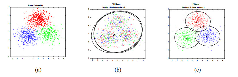
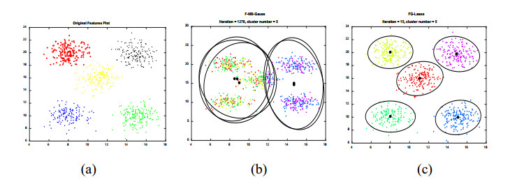
1. | Yulong Zhang, Ping Hu, Yaoyao Xie, Xiaoyu Wang, Co-fermentation with Lactobacillus curvatus LAB26 and Pediococcus pentosaceus SWU73571 for improving quality and safety of sour meat, 2020, 170, 03091740, 108240, 10.1016/j.meatsci.2020.108240 | |
2. | Dharmendra Kumar, Som Dutt, Pinky Raigond, Sushil Sudhakar Changan, Milan Kumar Lal, Devender Sharma, Brajesh Singh, 2020, Chapter 15, 978-981-15-7661-4, 271, 10.1007/978-981-15-7662-1_15 | |
3. | Irfan Khan, Saghir Ahmad, 2020, Chapter 14, 978-981-15-4715-7, 219, 10.1007/978-981-15-4716-4_14 | |
4. | Hélène Licandro, Phu Ha Ho, Thi Kim Chi Nguyen, Awanwee Petchkongkaew, Hai Van Nguyen, Son Chu-Ky, Thi Viet Anh Nguyen, Da Lorn, Yves Waché, How fermentation by lactic acid bacteria can address safety issues in legumes food products?, 2020, 110, 09567135, 106957, 10.1016/j.foodcont.2019.106957 | |
5. | Mira Serikkyzy, Gulzira Jumabekova, Ainur Zheldybayeva, Ainur Matibayeva, Roza Omirbay, Desislav Balev, Developing a Risk Assessment Methodology for the Production of Semi-Smoked Sausages, 2022, 1542-8052, 1, 10.1080/15428052.2022.2034695 | |
6. | Nur Anis Raihana Mhd Rodzi, Lai Kuan Lee, Traditional fermented foods as vehicle of non-dairy probiotics: Perspectives in South East Asia countries, 2021, 150, 09639969, 110814, 10.1016/j.foodres.2021.110814 | |
7. | Efe Sezgin, Burcu Tekin, Molecular evolution and population genetics of glutamate decarboxylase acid resistance pathway in lactic acid bacteria, 2023, 14, 1664-8021, 10.3389/fgene.2023.1027156 | |
8. | Michela Verni, Erica Pontonio, Marco Montemurro, Carlo Giuseppe Rizzello, 2022, Chapter 13, 978-1-80356-914-7, 10.5772/intechopen.102523 | |
9. | Mira Serikkyzy, Gulzira Jumabekova, Ainur Zheldybayeva, Ainur Matibayeva, Roza Omirbay, Desislav Balev, Improving the organoleptic and structural-chemical properties of semi-smoked sausages, 2022, 29, 1319562X, 1510, 10.1016/j.sjbs.2021.11.021 | |
10. | Ok Hee Choi, Won Il Kim, Dae Young Son, Ye Yeong Lee, Yong Sung Kang, Jin Woo Kim, Catalog of Lactic Acid Bacteria Associated with Vegetable Sprouts, 2023, 57, 1598-5504, 1, 10.14397/jals.2023.57.6.1 | |
11. | Fatma Beyza Özpınar, Hümeyra İspirli, Selma Kayacan, Kader Korkmaz, Sevda Dere, Osman Sagdic, Zuhal Alkay, Yunus Emre Tunçil, Mutamed Ayyash, Enes Dertli, Physicochemical and structural characterisation of a branched dextran type exopolysaccharide (EPS) from Weissella confusa S6 isolated from fermented sausage (Sucuk), 2024, 264, 01418130, 130507, 10.1016/j.ijbiomac.2024.130507 | |
12. | Sushmita Das, Maloyjo Joyraj Bhattacharjee, Ashis K. Mukherjee, Mojibur Rohman Khan, Selection of a multi-species starter culture for mustard seed fermentation to enhance polyunsaturated fatty acids and improve gastrointestinal health markers, 2024, 59, 22124292, 104109, 10.1016/j.fbio.2024.104109 | |
13. | Spiros Paramithiotis, Lactiplantibacillus plantarum, the Integral Member of Vegetable Fermentations, 2025, 4, 2813-0464, 7, 10.3390/applbiosci4010007 |
Channel | Wavelength (μm) | Waveband | Ground resolution (km) | Application |
AVHRR-1 | 0.58-0.68 | Visible light | 1.10 | Daytime clouds, ice, snow, vegetation |
AVHRR-2 | 0.725-1.10 | Near-infrared | 1.10 | Daytime clouds, vegetation, water, agricultural estimation, land usage survey |
AVHRR-3A | 1.58-1.64 | Middle-infrared | 1.10 | Daytime clouds, ice, snow, soil moisture, drought monitoring |
AVHRR-3B | 3.55-3.93 | Middle-infrared | 1.10 | Night clouds, forest fire, volcanic activity |
AVHRR-4 | 10.30-11.30 | Far-infrared | 1.10 | Day and night image, land surface temperature, sea surface temperature |
AVHRR-5 | 11.50-12.50 | Far- infrared | 1.10 | Day and night image, land surface temperature, sea surface temperature |
Remote sensing image | Support vector machine classification accuracy evaluation | |||
User’s accuracy | Commission error | Production accuracy | Omission error | |
Wet land | 87.62% | 12.38% | 99.28% | 0.72% |
Wasteland | 93.25% | 6.75% | 73.43% | 26.57% |
Crop | 81.55% | 18.5% | 84.85% | 15.15% |
Straw | 84.48% | 15.52% | 86.73% | 13.27% |
Overall accuracy | 87.52% | |||
Kappa coefficient | 0.8223 |
Remote sensing image | Radial basis function classification accuracy evaluation | |||
User’s accuracy | Commission error | Production accuracy | Omission error | |
Wet land | 83.45% | 16.55% | 83.16% | 16.84% |
Wasteland | 78.89% | 21.11% | 78.02% | 21.98% |
Crop | 83.43% | 16.57% | 82.82% | 17.18% |
Straw | 76.87% | 23.13% | 80.71% | 19.29% |
Overall accuracy | 82.01% | |||
Kappa coefficient | 0.7457 |
Remote sensing image | Improved convolutional neural network classification accuracy evaluation | |||
User’s accuracy | Commission error | Production accuracy | Omission error | |
Wet land | 97.86% | 2.14% | 98.92% | 1.08% |
Wasteland | 98.07% | 1.93% | 98.07% | 1.93% |
Crop | 97.94% | 2.06% | 95.96% | 4.04% |
Straw | 98.21% | 1.79% | 97.35% | 2.65% |
Overall accuracy | 97.99% | |||
Kappa coefficient | 0.9715 |