


Citation: Xiaoying Wang, Xingfu Zou. Pattern formation of a predator-prey model with the cost of anti-predator behaviors[J]. Mathematical Biosciences and Engineering, 2018, 15(3): 775-805. doi: 10.3934/mbe.2018035
| [1] | Chunmei Zhang, Suli Liu, Jianhua Huang, Weiming Wang . Stability and Hopf bifurcation in an eco-epidemiological system with the cost of anti-predator behaviors. Mathematical Biosciences and Engineering, 2023, 20(5): 8146-8161. doi: 10.3934/mbe.2023354 |
| [2] | Ceyu Lei, Xiaoling Han, Weiming Wang . Bifurcation analysis and chaos control of a discrete-time prey-predator model with fear factor. Mathematical Biosciences and Engineering, 2022, 19(7): 6659-6679. doi: 10.3934/mbe.2022313 |
| [3] | Yuanfu Shao . Bifurcations of a delayed predator-prey system with fear, refuge for prey and additional food for predator. Mathematical Biosciences and Engineering, 2023, 20(4): 7429-7452. doi: 10.3934/mbe.2023322 |
| [4] | Jinxing Zhao, Yuanfu Shao . Bifurcations of a prey-predator system with fear, refuge and additional food. Mathematical Biosciences and Engineering, 2023, 20(2): 3700-3720. doi: 10.3934/mbe.2023173 |
| [5] | Tingfu Feng, Leyun Wu . Global dynamics and pattern formation for predator-prey system with density-dependent motion. Mathematical Biosciences and Engineering, 2023, 20(2): 2296-2320. doi: 10.3934/mbe.2023108 |
| [6] | Saheb Pal, Nikhil Pal, Sudip Samanta, Joydev Chattopadhyay . Fear effect in prey and hunting cooperation among predators in a Leslie-Gower model. Mathematical Biosciences and Engineering, 2019, 16(5): 5146-5179. doi: 10.3934/mbe.2019258 |
| [7] | William Wolesensky, J. David Logan . An individual, stochastic model of growth incorporating state-dependent risk and random foraging and climate. Mathematical Biosciences and Engineering, 2007, 4(1): 67-84. doi: 10.3934/mbe.2007.4.67 |
| [8] | Yongli Cai, Malay Banerjee, Yun Kang, Weiming Wang . Spatiotemporal complexity in a predator--prey model with weak Allee effects. Mathematical Biosciences and Engineering, 2014, 11(6): 1247-1274. doi: 10.3934/mbe.2014.11.1247 |
| [9] | Yun Kang, Sourav Kumar Sasmal, Komi Messan . A two-patch prey-predator model with predator dispersal driven by the predation strength. Mathematical Biosciences and Engineering, 2017, 14(4): 843-880. doi: 10.3934/mbe.2017046 |
| [10] | Sourav Kumar Sasmal, Jeet Banerjee, Yasuhiro Takeuchi . Dynamics and spatio-temporal patterns in a prey–predator system with aposematic prey. Mathematical Biosciences and Engineering, 2019, 16(5): 3864-3884. doi: 10.3934/mbe.2019191 |
In ecological systems, spatially heterogeneous distributions of many species have been observed, for example, patchiness of plankton in aquatic systems [36]. Although such heterogeneity of species may be attributed to unevenly distributed landscapes, it may also occur in an almost homogeneous environment [36,19]. One interesting question is that what are the mechanisms behind the spatial heterogeneity of species in a homogeneous environment? Generally, movement or dispersal of a species and its interactions with other species may lead to pattern formation, and predator-prey type is such an interaction.
Pattern formation of predator-prey systems has been studied extensively (see [23,3,33,31,21,45,39,34] for example). In general, if both prey and predators move randomly in habitats, prey-dependent only functional responses, including the Holling type Ⅰ, Ⅱ, Ⅲ functional responses, can't generate spatially heterogeneous distributions. In such systems, the density-dependent death rate of predators or the Allee effect in prey's growth plays a critical role in determining spatial patterns [23,24,29,25,38,27,20]. On the other hand, competition between predators alone may allow pattern formation in predator-prey systems, which includes ratio-dependent functional response, the Beddington-DeAngelis functional response, and their generalizations [3,33,31]. Pattern formation of predator-prey models with time delay in the functional response due to handing time of the predator is also studied [47,44,9].
In addition to pure random movement of prey and predators, directed movement of predators has attracted much attention in recent years and has inspired numerous research about the so called prey-taxis problems (see [1,8,18,37,41,43,35] for example). A common feature of the models in the aforementioned papers lies in that the movement of predators is affected by the density gradient of prey, in addition to random movement. In analogy to the well-known chemotaxis, predators are attracted by prey-taxis and tend to move to habitats with higher prey density. Such biased movement allows predators to forage prey more effectively. In [1,37], the global existence of weak solution and classical solution were proved respectively. As an extension of [1,37], the authors in [43] proved the global existence of classical solution with more general local reaction terms and established the uniform persistence of the solutions as well. Global stability result of a predator-prey model with prey-taxis is obtained in recent work [17], where a broad range of growth and predation functions are considered. In [18], pattern formation was studied under various functional responses between prey and predators. The authors concluded that pattern formation may occur if the prey-taxis was small and certain functional responses or growth functions were chosen [18].
Besides the fact that predators forage prey, prey may avoid predators actively as well. Almost all species perceive predation risk to some extent and avoid predation by showing various anti-predator behaviors [10,11]. More importantly, such anti-predator behaviors carry a cost on the reproduction success of prey [46]. Zanette et al. [46] experimentally verified that anti-predator behaviors alone caused a
In this paper, we extend the model based on Wang et al.. by explicitly incorporating spatial effects, where spatial structures are ignored in [40]. We study how the anti-predator behaviors and the corresponding cost would affect the spatial distribution of prey and predators. In Section 2, the model formulation including the so-called predator-taxis is proposed. In Section 3, the global existence of classical solution is established. In Section 4, pattern formation is analyzed both theoretically and numerically for different functional responses. We end the paper in Section 5 by giving conclusions and discussions.
Let
| Ju=−du∇u−γ(u,v)u∇v, |
and the flux of predators is
| Jv=−dv∇v, |
where
| ut=∇⋅(du∇u+γ(u,v)u∇v)+f(u,v),vt=dvΔv+g(u,v), | (1) |
where
| γ(u,v)=β(u)α(v). | (2) |
Taking into account the volume filling effect [14,28,13] for
| β(u)={1−uM,if0≤u≤M,0,ifM<u, | (3) |
where
| f(u,v)=f0(k0α,v)r0u−du−au2−up(u,v)v,g(u,v)=v[−m(v)+cup(u,v)], | (4) |
where
| f0(k0α,v)=11+k0αv | (5) |
satisfies the same hypotheses as
| m(v)=m1orm(v)=m1+m2v. | (6) |
As indicated in [23,24,20], the density dependence of predator mortality plays a critical role in pattern formation under certain situations.
We assume that individuals live in an isolated bounded domain
| Ju⋅n=du∂u∂μ+γ(u,v)u∂v∂μ=0,Jv⋅n=dv∂v∂μ=0, | (7) |
where
| ∂u∂μ=0,∂v∂μ=0,∀x∈∂Ω. | (8) |
Therefore, by (1), (2), (4) and (8), we obtain a spatial model with the avoidance behaviors of prey and the cost of anti-predator behaviors, given by the following system
| ∂u∂t=duΔu+α∇⋅(β(u)u∇v)+r0u1+k0αv−du−au2−up(u,v)v,∂v∂t=dvΔv+v[−m(v)+cup(u,v)],∂u∂μ=0,∂v∂μ=0,∀x∈∂Ω,u(x,0)=u0(x)≥0,v(x,0)=v0(x)≥0, | (9) |
where
First, we establish the global existence of classical solutions of (9). It is clear that the carrying capacity of prey in (9) is
| M>r0−da, | (10) |
which is reasonable because
| ˉβ(u)={>1,u<0,β(u),0≤u≤M,<0,M<u. | (11) |
By proving the global existence of classical solutions of system
| ∂u∂t=duΔu+α∇⋅(ˉβ(u)u∇v)+r0u1+k0αv−du−au2−up(u,v)v,∂v∂t=dvΔv+v[−m(v)+cup(u,v)],∂u∂μ=0,∂v∂μ=0,∀x∈∂Ω,u(x,0)=u0(x)≥0,v(x,0)=v0(x)≥0, | (12) |
we obtain the global existence of classical solutions of (9) because
| X:={ω∈W1,ρ(Ω,R2)⏐∂ω∂μ=0on∂Ω}. |
Then we have the following lemma.
Lemma 3.1. The following statements hold:
(ⅰ) System (12) has a unique solution
(ⅱ) Define
Proof. Let
| {ωt=∇⋅(a(ω)∇ω)+F(ω)inΩ×(0,+∞),Bω=0on∂Ω×(0,+∞),ω(⋅,0)=(u0,v0)TinΩ, | (13) |
where
| a(ω)=(duαˉβ(u)u0dv), | (14) |
and
| F(ω)=(r0u1+k0αv−du−au2−up(u,v)v,v[−m(v)+cup(u,v)])T,Bω=∂ω∂n. | (15) |
Because eigenvalues of
From (ⅱ) of Lemma 3.1, to prove the global existence of solutions, it remains to show that
Theorem 3.2. Assume that
Proof. Define the operator
| Lu=ut−duΔu−α∇(ˉβ(u)u∇v)−r0u1+k0αv+du+au2+p(u,v)uv. | (16) |
Because
| LM=−r0M1+k0αv+dM+aM2+p(M,v)Mv=M(d+aM+p(M,v)v−r01+k0αv). | (17) |
If
| LM≥M(d+aM−r0). | (18) |
Because of the restriction (10), choosing sufficiently large
| LM≥0. | (19) |
In addition, we have
| ∂M∂μ=0,M≥u0. | (20) |
By (19) and (20), we know that
| 0≤u≤M. | (21) |
Now we prove the
| ∫Ωutdx=∫Ω∇⋅(du∇u+αˉβ(u)u∇v)dx+∫Ω(r0u1+k0αv−du−au2−p(u,v)uv)dx=∫∂Ω(du∇u+αˉβ(u)u∇v)⋅ndS+∫Ω(r0u1+k0αv−du−au2−p(u,v)uv)dx=∫Ω(r0u1+k0αv−du−au2−p(u,v)uv)dx. | (22) |
Similarly, integrating the second equation of (12) gives
| ∫Ωvtdx=∫Ωv[−m1+cp(u,v)u]dx. | (23) |
Multiplying (22) by
| ddt∫Ω(cu+v)dx=∫Ω(r0cu1+k0αv−cdu−cau2−m1v)dx=c∫Ω(r01+k0αv+m1−d−au)udx−m1∫Ω(cu+v)dx≤c∫Ω(r0+m1)udx−m1∫Ω(cu+v)dx≤c|Ω|(r0+m1)M−m1∫Ω(cu+v)dx. | (24) |
By (24), we obtain
| ddt‖cu+v‖L1≤c|Ω|(r0+m1)M−m1‖cu+v‖L1 | (25) |
From (25), we obtain that
| lim |
which shows that
Now we analyze the pattern formation of (9) with general reaction terms defined in (4). Assume that
| u(x, t) = u_s+\epsilon\, \tilde{u}(x, t), \;\;v(x, t) = v_s+\epsilon\, \tilde{v}(x, t), | (26) |
where
| \frac{\partial u}{\partial t} = d_u\, \Delta u+\alpha\, \beta(u_s)\, u_s\, \Delta v+f_u(u_s, v_s)\, u+f_v(u_s, v_s)\, v, \\ \frac{\partial v}{\partial t} = d_v\, \Delta v+g_u(u_s, v_s)\, u+g_v(u_s, v_s)\, v, | (27) |
where
| \frac{\partial \omega}{\partial t} = D\, \Delta \omega+A\, \omega, | (28) |
where
| \omega = \left(\begin{array}{c} u\\ v\\ \end{array}\right), \;\;\; D = \left( \begin {array}{cc} d_u&\alpha\, \beta(u_s)\, u_s\\ 0&d_v\\ \end {array} \right), \;\;\; A = \left( \begin {array}{cc} f_u&f_v\\ g_u&g_v\\ \end {array} \right). |
By (28), the characteristic polynomial of the linearized system at
| \vert \lambda\, \mathrm{I}+k^2\, D-A \vert = 0, | (29) |
where
| \lambda^2+a\left(k^2\right)\, \lambda+b\left(k^2\right) = 0, | (30) |
where
| a\left(k^2\right) = \left(d_u+d_v\right)k^2-\left(f_u+g_v\right), \\ b\left(k^2\right) = d_u\, d_v\, k^4+\left(g_u\, \alpha\, \beta(u_s)\, u_s-f_u\, d_v-g_v\, d_u\right)k^2+f_u\, g_v-f_v\, g_u. | (31) |
Here in (30),
| \lambda_1^0+\lambda_2^0 = f_u+g_v, \;\;\;\lambda_1^0\, \lambda_2^0 = f_u\, g_v-f_v\, g_u. | (32) |
Assume that
| f_u+g_v<0, \;f_u\, g_v-f_v\, g_u>0, | (33) |
meaning that the steady state
| \left\{ \begin{array}{l} \lambda _1^k + \lambda _2^k =\left( {{f_u} + {g_v}} \right) - \left( {{d_u} + {d_v}} \right){\mkern 1mu} {k^2}, \\ \lambda _1^k{\mkern 1mu} \lambda _2^k ={d_u}{\mkern 1mu} {d_v}{\mkern 1mu} {k^4} + \left( {{g_u}{\mkern 1mu} \alpha {\mkern 1mu} \beta ({u_s}){\mkern 1mu} {u_s} - {f_u}{\mkern 1mu} {d_v} - {g_v}{\mkern 1mu} {d_u}} \right){k^2} + {f_u}{\mkern 1mu} {g_v} - {f_v}{\mkern 1mu} {g_u}. \end{array} \right. | (34) |
Because of
Theorem 4.1. Assume (33) holds, spatial homogeneous steady state
| g_u\, \alpha\, \beta(u_s)\, u_s-f_u\, d_v-g_v\, d_u<0, | (35) |
| \left(g_u\, \alpha\, \beta(u_s)\, u_s-f_u\, d_v-g_v\, d_u\right)^2-4\, d_u\, d_v\, \left(f_u\, g_v-f_v\, g_u\right)>0 | (36) |
hold.
Remark 1. Under the assumption (33),
| g_u\, \alpha\, \beta(u_s)\, u_s>f_u\, d_v+g_v\, d_u. | (37) |
Following above general analysis of pattern formation of spatial homogeneous equilibrium, we now proceed to further detailed analysis when a particular functional response is chosen. First, we analyze possible pattern formation of (9) with the linear functional response, where
| r_0>d+\frac{a\, m_1}{c\, p} | (38) |
holds. However, formulas for
| \left\{ \begin{array}{l} \bar u =\frac{{{m_1}}}{{c{\mkern 1mu} p}}, \;\bar v =\frac{{\left( {\alpha {\mkern 1mu} c{\mkern 1mu} d{\mkern 1mu} {k_0}{\mkern 1mu} p + a{\mkern 1mu} \alpha {\mkern 1mu} {k_0}{\mkern 1mu} {m_1} + c{\mkern 1mu} {p^2}} \right) - \sqrt {{\Delta _1}} }}{{ - 2{\mkern 1mu} {k_0}{\mkern 1mu} \alpha {\mkern 1mu} {p^2}{\mkern 1mu} c}}, \\ {\Delta _1} =4{\mkern 1mu} \alpha {\mkern 1mu} c{\mkern 1mu} {k_0}{\mkern 1mu} {p^2}{\mkern 1mu} ( - c{\mkern 1mu} d{\mkern 1mu} p + c{\mkern 1mu} p{\mkern 1mu} {r_0} - a{\mkern 1mu} {m_1}) + {( - \alpha {\mkern 1mu} c{\mkern 1mu} d{\mkern 1mu} {k_0}{\mkern 1mu} p - a{\mkern 1mu} \alpha {\mkern 1mu} {k_0}{\mkern 1mu} {m_1} - c{\mkern 1mu} {p^2})^2} \end{array} \right. | (39) |
if
| \left\{ \begin{array}{l} \bar{v} = \frac{\left(c\, p^2+a\, m_2+k_0\, \alpha\, (d\, c\, p+a\, m_1)\right)-\sqrt{\Delta_2}}{-2\, k_0\, \alpha\, (c\, p^2+a\, m_2)}, \;\bar{u} = \frac{m_1+m_2\, \bar{v}}{c\, p}, \\ \Delta_2 = 4\, k_0\, \alpha\, (c\, p^2+a\, m_2)\, (-c\, d\, p+c\, p\, r_0-a\, m_1)\\ +(-\alpha\, c\, d\, k_0\, p-a\, \alpha\, k_0\, m_1-c\, p^2-a\, m_2)^2 \end{array} \right. | (40) |
if
Proposition 1. Either for
Proof. Because the proofs for all steady states are similar, we show only the proof of non-existence of pattern formation around
| {f_u} =- a{\mkern 1mu} \bar u < 0, \;{f_v} =\bar u{\mkern 1mu} \left( { - \frac{{{r_0}{\mkern 1mu} {k_0}{\mkern 1mu} \alpha }}{{{{(1 + {k_0}{\mkern 1mu} \alpha {\mkern 1mu} \bar v)}^2}}} - p} \right) < 0, \;{g_u} =c{\mkern 1mu} p{\mkern 1mu} \bar v, \;{g_v} =0. | (41) |
This immediately verifies (33), implying that
In fact, under additional conditions, we can prove that the unique positive equilibrium
Theorem 4.2. Under existence condition (38) for
| \left\{ \begin{array}{l} c\, p\, M>m_1, \;4\, d_u\, d_v\, \bar{v}>c\, \alpha^2\, \bar{u}\, {v^{*}}^2, \\ \min \left\{a, \frac{m_2}{c}\right\}>\frac{r_0\, k_0\, \alpha}{2\, (1+k_0\, \alpha\, \bar{v})} \end{array} \right. | (42) |
hold, where
Proof. As indicated in the proof of Lemma 3.1, the
| \mathcal{F}v = v_t-d_v\, \Delta v-v\, \left(-m_1-m_2\, v+c\, p\, u\right). | (43) |
Then by substituting
| \mathcal{F} v^{*} = -v^{*}\, \left(-m_1-m_2\, v^{*}+c\, p\, u\right) \geq 0 | (44) |
because
| V(u, v) = \int_{\Omega}\left( \int_{\bar{u}}^{u} \frac{u-\bar{u}}{u} du +\frac{1}{c} \int_{\bar{v}}^v \frac{v-\bar{v}}{v} dv \right)\, dx. | (45) |
If
| \begin{align}\label{lyapfun0} \frac{dV(u, v)}{dt}& = \int_{\Omega} \left(\frac{u-\bar{u}}{u} u_t+\frac{1}{c} \frac{v-\bar{v}}{v}v_t\right)dx \nonumber\\ & = \int_{\Omega} \frac{u-\bar{u}}{u} \Big(d_u\, \Delta u+\alpha \nabla \cdot(\beta(u)\, u\nabla v)+\frac{r_0\, u}{1+k_0\, \alpha\, v}-d\, u-a\, u^2 \nonumber\\ &-p\, u\, v\Big) dx\\ &+\frac{1}{c} \int_{\Omega}\frac{v-\bar{v}}{v} \left[d_v\, \Delta_v+v(-m_1-m_2\, v+c\, p\, u)\right] dx. \nonumber \end{align} | (46) |
Rearranging (46) by separating the reaction and dispersal terms gives
| \frac{dV(u, v)}{dt} = V_1(u, v)+V_2(u, v), | (47) |
where
| \begin{align}\label{V1V2} V_1(u, v)& = \int_{\Omega} \frac{u-\bar{u}}{u} \lbrack d_u\, \Delta u+\alpha \nabla \cdot(\beta(u)\, u\nabla v) \rbrack+ \frac{v-\bar{v}}{c\, v} d_v\, \Delta v \, dx, \nonumber\\ V_2(u, v)& = \int_{\Omega} (u-\bar{u})\left(\frac{r_0}{1+k_0\, \alpha\, v}-d-a\, u-p\, v\right) \\ &+\frac{v-\bar{v}}{c} (-m_1-m_2\, v+c\, p\, u) \, dx. \nonumber \end{align} | (48) |
By using Neumann boundary condition (8) and divergence theorem, we obtain that
| \begin{align}\label{V1} V_1(u, v)& = -d_u \int_{\Omega} \nabla \left(\frac{u-\bar{u}}{u}\right)\cdot \nabla u \, dx -\frac{d_v}{c}\int_{\Omega}\nabla v \cdot \, \nabla \left(\frac{v-\bar{v}}{v}\right)\, dx \nonumber\\ &-\alpha\int_{\Omega} \beta(u)\, u\, \nabla v\, \cdot \nabla \left(\frac{u-\bar{u}}{u}\right)\, dx \nonumber\\ &\leq -d_u\, \bar{u} \int_{\Omega} \frac{\vert \nabla u \vert^2}{u^2} \, dx-\frac{d_v\, \bar{v}}{c} \int_{\Omega} \frac{\vert \nabla v \vert^2}{v^2} \, dx +\alpha\, \bar{u} \int_{\Omega} \frac{\beta(u)}{u} \vert\nabla u\vert\, \vert\nabla v\vert\, dx \end{align} | (49) |
| = -\int_{\Omega} X^{\mathsf{T}}\, A\, X | (50) |
where
| X = \left(\begin{array}{c} \vert\nabla u\vert\\ \vert\nabla v\vert\\ \end{array}\right), \;\;\; A = \left( \begin {array}{cc} \displaystyle{ \frac{d_u\, \bar{u}}{u^2}}&\displaystyle -{\frac{\alpha\, \bar{u}\, \beta(u)}{2\, u}}\\ \displaystyle -{\frac{\alpha\, \bar{u}\, \beta(u)}{2\, u}}&\displaystyle{\frac{d_v\, \bar{v}}{c\, v^2}}\\ \end {array} \right).\;\;\; |
It is clear that
| \det{A} = \frac{d_u\, d_v\, \bar{u}\, \bar{v}}{c\, u^2\, v^2}-\frac{\alpha^2\, \bar{u}^2\, \beta^2(u)}{4\, u^2}. | (51) |
From (51), we obtain that
| 4\, d_u\, d_v\, \bar{v}>c\, \alpha^2\, \bar{u}\, v^2\, \beta^2(u). | (52) |
Because
| f_1: = 4\, d_u\, d_v\, \bar{v}>c\, \alpha^2\, \bar{u}\, {v^{*}}^2. | (53) |
Therefore, we obtain that
| V_1(u, v) = -\int_{\Omega} X^{\mathsf{T}}\, A\, X \leq 0 | (54) |
if (53) is satisfied.
Now we estimate
| \begin{align}\label{V2} V_2(u, v)& = \int_{\Omega} (u-\bar{u})\Bigg( \frac{r_0}{1+k_0\, \alpha\, v}-a\, u-p\, v-\left(\frac{r_0}{1+k_0\, \alpha\, \bar{v}}-a\, \bar{u}-p\, \bar{v}\right)\Bigg)\nonumber\\ &+\frac{v-\bar{v}}{c}\left(m_2\, \bar{v}-c\, p\, \bar{u}-m_2\, v+c\, p\, u\right)\, dx \nonumber \\ & = -a\, \int_{\Omega}(u-\bar{u})^2\, dx-\frac{m_2}{c}\int_{\Omega}(v-\bar{v})^2\, dx \nonumber \\ &-\int_{\Omega}\frac{r_0\, k_0\, \alpha}{1+k_0\, \alpha\, \bar{v}}\, \frac{(u-\bar{u})(v-\bar{v})}{1+k_0\, \alpha\, v}\, dx\\ &\leq -a\, \int_{\Omega}(u-\bar{u})^2\, dx-\frac{m_2}{c}\int_{\Omega}(v-\bar{v})^2\, dx \nonumber\\ &+\int_{\Omega}\frac{r_0\, k_0\, \alpha}{1+k_0\, \alpha\, \bar{v}}\, \frac{1}{1+k_0\, \alpha\, v}\, \vert(u-\bar{u})\vert \vert(v-\bar{v})\vert \, dx \nonumber \end{align} | (55) |
| \begin{align} &\leq -a\, \int_{\Omega}(u-\bar{u})^2\, dx-\frac{m_2}{c}\int_{\Omega}(v-\bar{v})^2\, dx \nonumber \\ &+\frac{r_0\, k_0\, \alpha}{2\, (1+k_0\, \alpha\, \bar{v})}\, \int_{\Omega} \left((u-\bar{u})^2+(v-\bar{v})^2\right)\, dx \nonumber \\ & = -\left(a-\frac{r_0\, k_0\, \alpha}{2\, (1+k_0\, \alpha\, \bar{v})}\right)\int_{\Omega}(u-\bar{u})^2\, dx \nonumber \\ &-\left(\frac{m_2}{c}-\frac{r_0\, k_0\, \alpha}{2\, (1+k_0\, \alpha\, \bar{v})}\right) \int_{\Omega} (v-\bar{v})^2\, dx \nonumber \\ &\leq 0 \end{align} | (56) |
if
| f_2: = \min \left\{a, \frac{m_2}{c}\right\}>\frac{r_0\, k_0\, \alpha}{2\, (1+k_0\, \alpha\, \bar{v})} | (57) |
holds. From (55), under (57), the only possibility such that
By checking conditions in (42), we can not obtain an explicit formula for the predator-taxis sensitivity
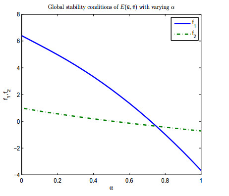 Figure 1. Conditions of global stability of
 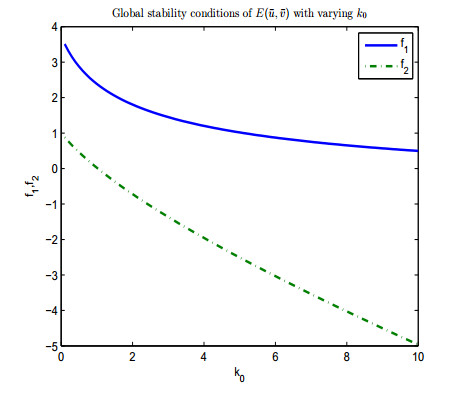 Figure 2. Conditions of global stability of
 Now we analyze possible pattern formation of system (9) with the Holling type Ⅱ functional response [15,16] i.e.,
| p(u, v) = \frac{p}{1+q\, u}. | (58) |
For general death function of predators defined in (6), a trivial equilibrium
| c\, p>m_1\, q \,\,\,\,\,\,\mbox{and}\,\,\,\,\,\, r_0-d>\frac{a\, m_1}{c\, p-m_1\, q} | (59) |
hold, where
| \begin{align}\label{holling2posiuv} \bar{u}& = \frac{m_1}{c\, p-m_1\, q}, \;\bar{v} = \frac{-a_2-\sqrt{a_2^2-4\, a_1\, a_3}}{2\, a_1}, \nonumber \\ a_1& = -k_0\, \alpha\, (c\, p-m_1\, q)^2, \nonumber \\ a_2& = -\alpha\, c^2\, d\, k_0\, p +\alpha\, c\, d\, k_0\, m_1\, q-a\, \alpha\, c\, k_0\, m_1-c^2\, p^2+2\, c\, m_1\, p\, q-m_1^2\, q^2, \\ a_3& = -c\, (c\, d\, p-c\, p\, r_0-d\, m_1\, q+m_1\, q\, r_0+a\, m_1). \nonumber \end{align} | (60) |
Calculations indicate that pattern formation can not occur around any of these steady states
Proposition2. Choose the functional response in (58) for (9). If the death function of predators is density-independent, then pattern formation can not occur around all the steady states
Proof. Here we only show the proof for the unique positive equilibrium
| f_u = \bar{u}\left(\frac{p\, q\, \bar{v}}{(1+q\, \bar{u})^2}-a\right), \; f_v = -\frac{r_0\, k_0\, \alpha\, \bar{u}}{(1+k_0\, \alpha\, \bar{v})^2}-\frac{p\, \bar{u}}{1+q\, \bar{u}}, \\ g_u = \frac{c\, p\, \bar{v}}{(1+q\, \bar{u})^2}, \;g_v = -m_1+\frac{c\, p\, \bar{u}}{1+q\, \bar{u}}. | (61) |
By substituting
Now we proceed to analyze the case where the death function of predators is the density-dependent one in (6). Similar analyses to that in Proposition 2 show that there is no pattern formation around
Lemma 4.3. If
Proof. From (9), the positive equilibrium
| \bar{u} = \frac{m_1+m_2\, \bar{v}}{(c\, p-m_1\, q)-m_2\, q\, \bar{v}}. | (62) |
By (62), the positivity of
| \bar{v}_{\max} = \frac{(c\, p-m_1\, q)}{m_2\, q}. | (63) |
In addition,
| L(\bar{v}): = a_1\, \bar{v}^4+a_2\, \bar{v}^3+a_3\, \bar{v}^2+a_4\, \bar{v}+a_5 = 0, | (64) |
where
| \begin{align} a_1& = -\alpha\, k_0\, m_2^2\, q^2, \;a_2 = m_2\, q\, (2\, \alpha\, c\, k_0\, p-2\, \alpha\, k_0\, m_1\, q-m_2\, q), \nonumber \\ a_3& = -(c^2\, p^2+((-d\, m_2-2\, m_1\, p)\, q+a\, m_2)\, c+q^2\, m_1^2)\, k_0\, \alpha+2\, q\, m_2\, (c\, p-m_1\, q), \nonumber\\ a_4& = (-\alpha\, d\, k_0\, p-p^2)\, c^2+(((\alpha\, d\, k_0+2\, p)\, m_1+m_2\, (d-r_0))\, q\\ &-a\, (\alpha\, k_0\, m_1+m_2))\, c -q^2\, m_1^2, \nonumber \\ a_5& = -c\, ((-d\, q+q\, r_0+a)\, m_1+c\, p\, (d-r_0)). \nonumber \end{align} | (65) |
By substituting
| L(\bar{v} = 0) = a_5>0 \Leftrightarrow (c\, p-m_1\, q)(r_0-d)>a\, m_1, | (66) |
which is equivalent to (59). Moreover, substituting
| L(\bar{v} = \bar{v}_{\max}) = -\frac{a\, c^2\, p\, (\alpha\, c\, k_0\, p-\alpha\, k_0\, m_1\, q+m_2\, q)}{m_2\, q^2}<0 | (67) |
if (59) holds. Therefore, by the intermediate value theorem, there exists at least one
When
 Figure 3. Spatial homogeneous steady states of
  Figure 4. Spatial heterogeneous steady states of
 In this section, we analyze (9) with the ratio-dependent functional response, i.e.
| p(u, v) = \frac{b_1}{b_2\, v+u} | (68) |
again with the predator death rate functions given in (6). For either death function of predators, system (9) with (68) admits a spatial homogeneous semi-trivial equilibrium
Consider the case with
| c\, b_1>m_1\,\,\,\,\, \mbox{and}\,\,\,\,\, r_0-d>\frac{c\, b_1-m_1}{c\, b_2}, | (69) |
where
| \left\{ \begin{array}{l} \bar{u} = \frac{m_1\, b_2\, \bar{v}}{c\, b_1-m_1}, \;\bar{v} = \frac{-a_2-\sqrt{a_2^2-4\, a_1\, a_3}}{2\, a_1}, \\ a_1 = -k_0\, \alpha\, a\, m_1\, b_2^2\, c, \\ a_2 = -k_0\, \alpha\, (m_1-c\, b_1)^2-c\, b_2\, \left(a\, m_1\, b_2+k_0\, \alpha\, d\, (c\, b_1-m_1)\right), \\ a_3 = -(c\, b_1-m_1)\left((c\, b_1-m_1)+c\, b_2\, (d-r_0)\right). \end{array} \right. | (70) |
Assume
| \bar{u} = \frac{c\, b_2\, (r_0-d)-(c\, b_1-m_1)}{b_2\, a\, c}, \;\bar{v} = \frac{(c\, b_1-m_1)\left(c\, b_2\, (r_0-d)-(c\, b_1-m_1)\right)}{a\, m_1\, c\, b_2^2}, | (71) |
which do not involve
Proposition 3. When (69) holds and
| \begin{align} r_0-d>\frac{(c\, b_1-m_1)(c\, b_1+m_1-c\, b_2\, m_1)}{b_1\, b_2\, c^2}, \end{align} | (72) |
| \alpha<\frac{f_u\, d_v+g_v\, d_u-2\, \sqrt{d_u\, d_v\, \left(f_u\, g_v-f_v\, g_u\right)}}{g_u\, \beta(\bar{u})\, \bar{u}} | (73) |
hold.
Proof. Direct calculations show that at
| f_u = \bar{u}\left(-a+\frac{b_1\, \bar{v}}{(b_2\, \bar{v}+\bar{u})^2}\right), \; f_v = \bar{u}\, \left(-\frac{b_1}{b_2\, \bar{v}+\bar{u}} +\frac{b_1\, b_2\, \bar{v}}{(b_2\, \bar{v}+\bar{u})^2}\right), \\ g_u = \frac{c\, b_1\, b_2\, \bar{v}^2}{(b_2\, \bar{v}+\bar{u})^2}, \;g_v = -\frac{c\, b_1\, b_2\, \bar{u}\, \bar{v}}{(b_2\, \bar{v}+\bar{u})^2}. | (74) |
Substituting (74) into (35) and (36) gives
| \left\{ \begin{array}{l} \alpha<\frac{f_u\, d_v+g_v\, d_u}{g_u\, \beta(\bar{u})\bar{u}}, \\ \alpha<\frac{f_u\, d_v+g_v\, d_u-2\, \sqrt{d_u\, d_v\, \left(f_u\, g_v-f_v\, g_u\right)}}{g_u\, \beta(\bar{u})\, \bar{u}}, \end{array} \right. | (75) |
which leads to (73). Moreover, (33) needs to be satisfied to guarantee the local stability of
Proposition 3 implies that when there is no cost of anti-predator defense on the reproduction success of prey, small predator-taxis sensitivity
| \alpha_c = \frac{f_u\, d_v+g_v\, d_u-2\, \sqrt{d_u\, d_v\, \left(f_u\, g_v-f_v\, g_u\right)}}{g_u\, \beta(\bar{u})\, \bar{u}}. | (76) |
By choosing parameter values as shown in Figure 5 and substituting them into (76), we obtain the critical value of bifurcation
| k_1^2 < k^2<k_2^2 | (77) |
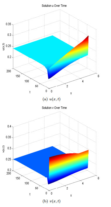 Figure 5. Spatial homogeneous steady states of
 where
| k_1^2 = \frac{-\left(g_u\, \alpha\, \beta(\bar{u})\bar{u}-f_u\, d_v-g_v\, d_u\right)-\sqrt{\Delta}}{2\, d_u\, d_v}, \\ k_2^2 = \frac{-\left(g_u\, \alpha\, \beta(\bar{u})\bar{u}-f_u\, d_v-g_v\, d_u\right)+\sqrt{\Delta}}{2\, d_u\, d_v}, \\ \Delta = \left(g_u\, \alpha\, \beta(\bar{u})\, \bar{u}-f_u\, d_v-g_v\, d_u\right)^2-4\, d_u\, d_v\, \left(f_u\, g_v-f_v\, g_u\right).\\ | (78) |
Equivalently, (77) in terms of modes
| n_1^2<n^2<n_2^2, | (79) |
where
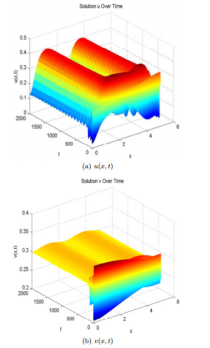 Figure 6.
Spatial heterogenous steady states of
Figure 6.
Spatial heterogenous steady states of Now we analyze the case where
| \left\{ \begin{array}{l} \alpha>\alpha_1 = 0.2979, \\ \alpha>\alpha_2 = 0.5277\;\text{or}\;\alpha<\alpha_3 = 0.1833 \end{array} \right. | (80) |
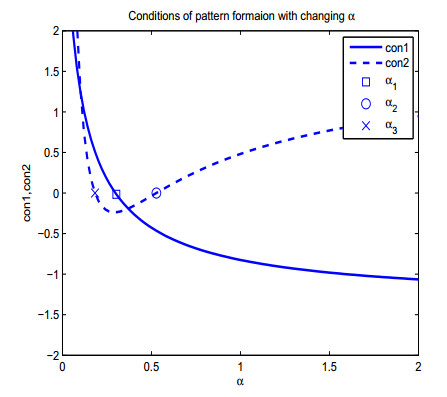 Figure 7. Conditions of diffusion-taxis-driven instability of
 to ensure the pattern formation of
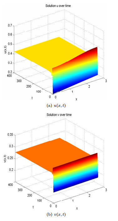 Figure 8. Spatial homogeneous steady states of
  Figure 9. Spatial heterogenous steady states of
 By comparing the two cases where
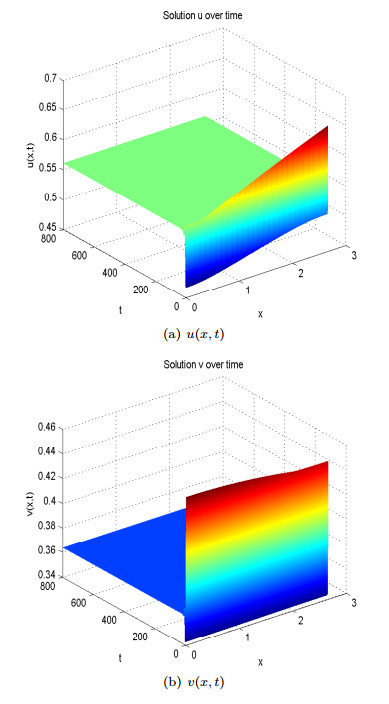 Figure 10. Spatial homogeneous steady states of
 We also point out here that in [3], the authors analyzed pattern formation of a predator-prey system where both prey and predators disperse randomly. By using numerical simulations, and considering the same ratio-dependent functional response, the authors concluded that the most possible Turing pattern occurred at places where the growth rate of prey and the death rate of predators were similar [3]. As a special case of (9), we also analyze the model
| \frac{\partial u}{\partial t} = d_u\, \Delta u+\frac{r_0\, u}{1+k_0\, \alpha\, v}-d\, u-a\, u^2-\frac{b_1\, u\, v}{b_2\, v+u}, \\ \frac{\partial v}{\partial t} = d_v\, \Delta v+v\left(-m_1+\frac{c\, b_1\, u}{b_2\, v+u}\right).\\ | (81) |
As shown in (81), different from model (9), prey have no directed movement but disperse randomly in the habitat. However, in local reaction between prey and predators, the cost of anti-predator behaviors still exists and the reproduction success of prey is reduced as a result. For notational convenience, let
Now we proceed to the case where the death function of predators is density dependent, where
Lemma 4.4. If
Proof. From (9), it is obvious that
| \bar{u} = \frac{b_2\, \bar{v}\, (m_2\, \bar{v}+m_1)}{(b_1\, c-m_1)-m_2\, \bar{v}}. | (82) |
Obviously, the existence of
| \bar{v}<\frac{b_1\, c-m_1}{m_2}: = \bar{v}_{\max}, | (83) |
where
| F(\bar{v}): = a_1\, \bar{v}^3+a_2\, \bar{v}^2+a_3\, \bar{v}+a_4 = 0, | (84) |
where
| \begin{align}\label{coeffr} a_1& = -\alpha\, k_0\, m_2\, (a\, b_2^2\, c+m_2), \nonumber \\ a_2& = -m_2^2+(((b_2\, d+2\, b_1)\, c-2\, m_1)\, k_0\, \alpha-a\, b_2^2\, c) \, m_2-a\, \alpha\, b_2^2\, c\, k_0\, m_1, \nonumber \\ a_3& = -\alpha\, b_1\, k_0\, (b_2\, d+b_1)\, c^2+(k_0\, m_1\, (b_2\, d+2\, b_1)\, \alpha -a\, b_2^2\, m_1\\ &+m_2\, (d-r_0)\, b_2+2\, b_1\, m_2)\, c-\alpha\, k_0\, m_1^2-2\, m_1\, m_2, \nonumber \\ a_4& = -(b_1\, c-m_1)\, (b_2\, c\, d-b_2\, c\, r_0+b_1\, c-m_1). \nonumber \end{align} | (85) |
From (85),
| (r_0-d)\, b_2\, c>b_1\, c-m_1, | (86) |
which is implied by (69). Furthermore, substituting
| F(\bar{v}_{\max}) = -\frac{a\, b_1\, b_2^2\, c^2\, (b_1\, c-m_1)\, (\alpha\, b_1\, c\, k_0-\alpha\, k_0\, m_1+m_2)}{m_2^2}<0 | (87) |
if
When
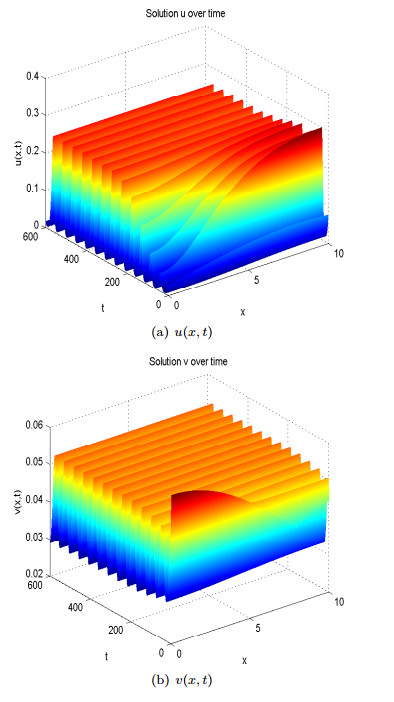 Figure 11. Spatial homogeneous but temporal periodic solution
 In this section, we analyze possible pattern formation when
| p(u, v) = \frac{p}{1+q_1\, u+q_2\, v}. | (88) |
For either death function
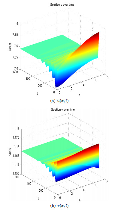 Figure 12. Spatial homogeneous steady states of
 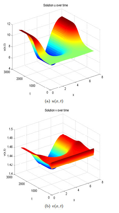 Figure 13. Spatial heterogeneous steady states of
 In this paper, we propose a spatial predator-prey model with avoidance behaviors in the prey as well as the corresponding cost of anti-predator responses on the reproduction success of prey. The focus is on the formation of spatial patterns. Various functional responses and both density-independent and density-dependent death rates of predators are considered for the model.
Mathematical analyses show that pattern formation cannot occur if the functional response is linear, or it is the Holling type Ⅱ but the death rate of the predators is density-independent. However, pattern formation may occur if the death rate of predators is density-dependent with the Holling type Ⅱ functional response. Moreover, functional responses other than the prey-dependent only ones, including ratio-dependent functional response and the Beddington-DeAngelis functional response, may also allow the emergence of spatial heterogeneous patterns. Under conditions for pattern formation, the common point for the case with the Holling type Ⅱ functional response and the case where the functional response is chosen as the Beddington-DeAngelis type is that small prey sensitivity to predation risk (i.e. small
In this paper, we mainly focused on modelling avoidance behaviors and the cost of anti-predator behaviors in the reproduction of prey in a spatial predator-prey system. Therefore, predators are assumed to move randomly in their habitats. In reality some predator species demonstrate prey-taxi when they forage for their preys (see, e.g., [43]). It is interesting to see how the prey-taxis effect on the predators and the predator-taxi effect on the prey (fear effect) will jointly affect the population dynamics in the predator-prey system. A even more interesting question would be how these two types of taxi effects will interplay with the cost of anti-predator behaviors. We leave these as possible future work.
The authors would like to thank Dr. Yixiang Wu for his reading and commenting on the manuscript, which helped us to improve the presentation of the paper. The authors also thank two anonymous reviewers for their careful reading and valuable feedback.
| [1] | [ B. E. Ainseba,M. Bendahmane,A. Noussair, A reaction-diffusion system modeling predator-prey with prey-taxis, Nonlinear Analysis: Real World Applications, 9 (2008): 2086-2105. |
| [2] | [ N. D. Alikakos, An application of the invariance principle to reaction-diffusion equations, Journal of Differential Equations, 33 (1979): 201-225. |
| [3] | [ D. Alonso,F. Bartumeus,J. Catalan, Mutual interference between predators can give rise to Turing spatial patterns, Ecology, 83 (2002): 28-34. |
| [4] | [ H. Amann, Dynamic theory of quasilinear parabolic equations Ⅱ: Reaction-diffusion systems, Differential Integral Equations, 3 (1990): 13-75. |
| [5] | [ H. Amann, Dynamic theory of quasilinear parabolic systems Ⅲ: Global existence, Mathematische Zeitschrift, 202 (1989): 219-250. |
| [6] | [ H. Amann, Nonhomogeneous linear and quasilinear elliptic and parabolic boundary value problems, Function Spaces, Differential Operators and Nonlinear Analysis, 133 (1993): 9-126. |
| [7] | [ J. R. Beddington, Mutual interference between parasites or predators and its effect on searching efficiency, Journal of Animal Ecology, 44 (1975): 331-340. |
| [8] | [ V. N. Biktashev,J. Brindley,A. V. Holden,M. A. Tsyganov, Pursuit-evasion predator-prey waves in two spatial dimensions, Chaos: An Interdisciplinary Journal of Nonlinear Science, 14 (2004): 988-994. |
| [9] | [ X. Cao, Y. Song and T. Zhang, Hopf bifurcation and delay-induced Turing instability in a diffusive lac operon model, International Journal of Bifurcation and Chaos, 26 (2016), 1650167, 22pp. |
| [10] | [ S. Creel,D. Christianson, Relationships between direct predation and risk effects, Trends in Ecology & Evolution, 23 (2008): 194-201. |
| [11] | [ W. Cresswell, Predation in bird populations, Journal of Ornithology, 152 (2011): 251-263. |
| [12] | [ D. L. DeAngelis,R. A. Goldstein,R. V. O'neill, A model for tropic interaction, Ecology, 56 (1975): 881-892. |
| [13] | [ T. Hillen,K. J. Painter, A user's guide to PDE models for chemotaxis, Journal of Mathematical Biology, 58 (2009): 183-217. |
| [14] | [ T. Hillen,K. J. Painter, Global existence for a parabolic chemotaxis model with prevention of overcrowding, Advances in Applied Mathematics, 26 (2001): 280-301. |
| [15] | [ C. S. Holling, The components of predation as revealed by a study of small-mammal predation of the European pine sawfly, The Canadian Entomologist, 91 (1959): 293-320. |
| [16] | [ C. S. Holling, Some characteristics of simple types of predation and parasitism, The Canadian Entomologist, 91 (1959): 385-398. |
| [17] | [ H. Jin,Z. Wang, Global stability of prey-taxis systems, Journal of Differential Equations, 262 (2017): 1257-1290. |
| [18] | [ J. M. Lee,T. Hillen,M. A. Lewis, Pattern formation in prey-taxis systems, Journal of Biological Dynamics, 3 (2009): 551-573. |
| [19] | [ S. A. Levin, The problem of pattern and scale in ecology, Ecology, 73 (1992): 1943-1967. |
| [20] | [ E. A. McGehee,E. Peacock-López, Turing patterns in a modified Lotka-Volterra model, Physics Letters A, 342 (2005): 90-98. |
| [21] | [ A. B. Medvinsky,S. V. Petrovskii,I. A. Tikhonova,H. Malchow,B. Li, Spatiotemporal complexity of plankton and fish dynamics, SIAM Review, 44 (2002): 311-370. |
| [22] | [ J. D. Meiss, Differential Dynamical Systems, SIAM, 2007. |
| [23] | [ M. Mimura,J. D. Murray, On a diffusive prey-predator model which exhibits patchiness, Journal of Theoretical Biology, 75 (1978): 249-262. |
| [24] | [ M. Mimura, Asymptotic behavior of a parabolic system related to a planktonic prey and predator system, SIAM Journal on Applied Mathematics, 37 (1979): 499-512. |
| [25] | [ A. Morozov,S. Petrovskii,B. Li, Spatiotemporal complexity of patchy invasion in a predator-prey system with the Allee effect, Journal of Theoretical Biology, 238 (2006): 18-35. |
| [26] | [ J. D. Murray, Mathematical Biology Ⅱ: Spatial Models and Biomedical Applications, Third edition. Interdisciplinary Applied Mathematics, 18. Springer-Verlag, New York, 2003. |
| [27] | [ W. Ni,M. Wang, Dynamics and patterns of a diffusive Leslie-Gower prey-predator model with strong Allee effect in prey, Journal of Differential Equations, 261 (2016): 4244-4274. |
| [28] | [ K. J. Painter,T. Hillen, Volume-filling and quorum-sensing in models for chemosensitive movement, Can. Appl. Math. Quart, 10 (2002): 501-543. |
| [29] | [ S. V. Petrovskii,A. Y. Morozov,E. Venturino, Allee effect makes possible patchy invasion in a predator-prey system, Ecology Letters, 5 (2002): 345-352. |
| [30] | [ D. Ryan,R. Cantrell, Avoidance behavior in intraguild predation communities: A cross-diffusion model, Discrete and Continuous Dynamical Systems, 35 (2015): 1641-1663. |
| [31] | [ H. Shi,S. Ruan, Spatial, temporal and spatiotemporal patterns of diffusive predator-prey models with mutual interference, IMA Journal of Applied Mathematics, 80 (2015): 1534-1568. |
| [32] | [ H. L. Smith, Monotone Dynamical Systems: An Introduction to the Theory of Competitive and Cooperative Systems, Mathematical Surveys and Monographs, 41. American Mathematical Society, Providence, RI, 1995. |
| [33] | [ Y. Song,X. Zou, Spatiotemporal dynamics in a diffusive ratio-dependent predator-prey model near a Hopf-Turing bifurcation point, Computers and Mathematics with Applications, 37 (2014): 1978-1997. |
| [34] | [ Y. Song,T. Zhang,Y. Peng, Turing-Hopf bifurcation in the reaction-diffusion equations and its applications, Communications in Nonlinear Science and Numerical Simulation, 33 (2016): 229-258. |
| [35] | [ Y. Song and X. Tang, Stability, steady-state bifurcations, and Turing patterns in a predator-prey model with herd behavior and prey-taxis, Studies in Applied Mathematics,(2017). |
| [36] | [ J. H. Steele, Spatial Pattern in Plankton Communities (Vol. 3), Springer Science & Business Media, 1978. |
| [37] | [ Y. Tao, Global existence of classical solutions to a predator-prey model with nolinear prey-taxis, Nonlinear Analysis: Real World Applications, 11 (2010): 2056-2064. |
| [38] | [ J. Wang,J. Shi,J. Wei, Dynamics and pattern formation in a diffusive predator-prey system with strong Allee effect in prey, Journal of Differential Equations, 251 (2011): 1276-1304. |
| [39] | [ J. Wang,J. Wei,J. Shi, Global bifurcation analysis and pattern formation in homogeneous diffusive predator-prey systems, Journal of Differential Equations, 260 (2016): 3495-3523. |
| [40] | [ X. Wang,L. Y. Zanette,X. Zou, Modelling the fear effect in predator-prey interactions, Journal of Mathematical Biology, 73 (2016): 1179-1204. |
| [41] | [ X. Wang,W. Wang,G. Zhang, Global bifurcation of solutions for a predator-prey model with prey-taxis, Mathematical Methods in the Applied Sciences, 38 (2015): 431-443. |
| [42] | [ Z. Wang and T. Hillen, Classical solutions and pattern formation for a volume filling chemotaxis model, Chaos: An Interdisciplinary Journal of Nonlinear Science, 17 (2007), 037108, 13 pp. |
| [43] | [ S. Wu,J. Shi,B. Wu, Global existence of solutions and uniform persistence of a diffusive predator-prey model with prey-taxis, Journal of Differential Equations, 260 (2016): 5847-5874. |
| [44] | [ J. Xu,G. Yang,H. Xi,J. Su, Pattern dynamics of a predator-prey reaction-diffusion model with spatiotemporal delay, Nonlinear Dynamics, 81 (2015): 2155-2163. |
| [45] | [ F. Yi,J. Wei,J. Shi, Bifurcation and spatiotemporal patterns in a homogeneous diffusive predator-prey system, Journal of Differential Equations, 246 (2009): 1944-1977. |
| [46] | [ L. Y. Zanette,A. F. White,M. C. Allen,M. Clinchy, Perceived predation risk reduces the number of offspring songbirds produce per year, Science, 334 (2011): 1398-1401. |
| [47] | [ T. Zhang and H. Zang, Delay-induced Turing instability in reaction-diffusion equations, Physical Review E, 90 (2014), 052908. |
| 1. | Kejun Zhuang, Hongjun Yuan, Spatiotemporal dynamics of a predator–prey system with prey-taxis and intraguild predation, 2019, 2019, 1687-1847, 10.1186/s13662-019-1945-3 | |
| 2. | Swati Mishra, Ranjit Kumar Upadhyay, Strategies for the existence of spatial patterns in predator–prey communities generated by cross-diffusion, 2020, 51, 14681218, 103018, 10.1016/j.nonrwa.2019.103018 | |
| 3. | Yang Wang, Xingfu Zou, On a Predator–Prey System with Digestion Delay and Anti-predation Strategy, 2020, 30, 0938-8974, 1579, 10.1007/s00332-020-09618-9 | |
| 4. | RENJI HAN, LAKSHMI NARAYAN GUIN, BINXIANG DAI, CROSS-DIFFUSION-DRIVEN PATTERN FORMATION AND SELECTION IN A MODIFIED LESLIE–GOWER PREDATOR–PREY MODEL WITH FEAR EFFECT, 2020, 28, 0218-3390, 27, 10.1142/S0218339020500023 | |
| 5. | Pingping Cong, Meng Fan, Xingfu Zou, Dynamics of a three-species food chain model with fear effect, 2021, 99, 10075704, 105809, 10.1016/j.cnsns.2021.105809 | |
| 6. | Sainan Wu, Jinfeng Wang, Junping Shi, Dynamics and pattern formation of a diffusive predator–prey model with predator-taxis, 2018, 28, 0218-2025, 2275, 10.1142/S0218202518400158 | |
| 7. | Sourav Kumar Sasmal, Population dynamics with multiple Allee effects induced by fear factors – A mathematical study on prey-predator interactions, 2018, 64, 0307904X, 1, 10.1016/j.apm.2018.07.021 | |
| 8. | Feng Dai, Bin Liu, Global solution for a general cross-diffusion two-competitive-predator and one-prey system with predator-taxis, 2020, 89, 10075704, 105336, 10.1016/j.cnsns.2020.105336 | |
| 9. | Vikas Kumar, Nitu Kumari, Stability and Bifurcation Analysis of Hassell–Varley Prey–Predator System with Fear Effect, 2020, 6, 2349-5103, 10.1007/s40819-020-00899-y | |
| 10. | Xinxin Guo, Jinfeng Wang, Dynamics and pattern formations in diffusive predator‐prey models with two prey‐taxis, 2019, 42, 0170-4214, 4197, 10.1002/mma.5639 | |
| 11. | A. V. Budyansky, V. G. Tsybulin, Modeling of Multifactor Taxis in a Predator–Prey System, 2019, 64, 0006-3509, 256, 10.1134/S0006350919020040 | |
| 12. | Vandana Tiwari, Jai Prakash Tripathi, Swati Mishra, Ranjit Kumar Upadhyay, Modeling the fear effect and stability of non-equilibrium patterns in mutually interfering predator–prey systems, 2020, 371, 00963003, 124948, 10.1016/j.amc.2019.124948 | |
| 13. | Ao Li, Xingfu Zou, Evolution and Adaptation of Anti-predation Response of Prey in a Two-Patchy Environment, 2021, 83, 0092-8240, 10.1007/s11538-021-00893-5 | |
| 14. | Jiang Li, Xiaohui Liu, Chunjin Wei, The impact of fear factor and self-defence on the dynamics of predator-prey model with digestion delay, 2021, 18, 1551-0018, 5478, 10.3934/mbe.2021277 | |
| 15. | Cuihua Wang, Sanling Yuan, Hao Wang, Spatiotemporal patterns of a diffusive prey-predator model with spatial memory and pregnancy period in an intimidatory environment, 2022, 84, 0303-6812, 10.1007/s00285-022-01716-4 | |
| 16. | Xiaoying Wang, Alexander Smit, Studying the fear effect in a predator-prey system with apparent competition, 2023, 28, 1531-3492, 1393, 10.3934/dcdsb.2022127 | |
| 17. | Xiaoyan Gao, Global Solution and Spatial Patterns for a Ratio-Dependent Predator–Prey Model with Predator-Taxis, 2022, 77, 1422-6383, 10.1007/s00025-021-01595-z | |
| 18. | Jianzhi Cao, Fang Li, Pengmiao Hao, Steady states of a diffusive predator-prey model with prey-taxis and fear effect, 2022, 2022, 1687-2770, 10.1186/s13661-022-01685-z | |
| 19. | Swati Mishra, Ranjit Kumar Upadhyay, 2022, Chapter 14, 978-3-030-81169-3, 147, 10.1007/978-3-030-81170-9_14 | |
| 20. | Jonathan Bell, Evan C. Haskell, Attraction–repulsion taxis mechanisms in a predator–prey model, 2021, 2, 2662-2963, 10.1007/s42985-021-00080-0 | |
| 21. | Zainab Saeed Abbas, Raid Kamel Naji, Modeling and Analysis of the Influence of Fear on a Harvested Food Web System, 2022, 10, 2227-7390, 3300, 10.3390/math10183300 | |
| 22. | Heather Banda, Michael Chapwanya, Phindile Dumani, Pattern formation in the Holling–Tanner predator–prey model with predator-taxis. A nonstandard finite difference approach, 2022, 196, 03784754, 336, 10.1016/j.matcom.2022.01.028 | |
| 23. | Xuebing Zhang, Hongyong Zhao, Yuan Yuan, Impact of discontinuous harvesting on a diffusive predator–prey model with fear and Allee effect, 2022, 73, 0044-2275, 10.1007/s00033-022-01807-8 | |
| 24. | Renji Han, Gergely Röst, Stationary and oscillatory patterns of a food chain model with diffusion and predator‐taxis, 2023, 0170-4214, 10.1002/mma.9079 | |
| 25. | Jia Liu, Qualitative analysis of a diffusive predator–prey model with Allee and fear effects, 2021, 14, 1793-5245, 2150037, 10.1142/S1793524521500376 | |
| 26. | Swati Mishra, Ranjit Kumar Upadhyay, Exploring the cascading effect of fear on the foraging activities of prey in a three species Agroecosystem, 2021, 136, 2190-5444, 10.1140/epjp/s13360-021-01936-5 | |
| 27. | Sharada Nandan Raw, Barsa Priyadarsini Sarangi, Dynamics of a diffusive food chain model with fear effects, 2021, 137, 2190-5444, 10.1140/epjp/s13360-021-02244-8 | |
| 28. | Xuebing Zhang, Honglan Zhu, Qi An, Dynamics analysis of a diffusive predator-prey model with spatial memory and nonlocal fear effect, 2023, 525, 0022247X, 127123, 10.1016/j.jmaa.2023.127123 | |
| 29. | Xuebing Zhang, Qi An, Ling Wang, Spatiotemporal dynamics of a delayed diffusive ratio-dependent predator–prey model with fear effect, 2021, 105, 0924-090X, 3775, 10.1007/s11071-021-06780-x | |
| 30. | EVAN C. HASKELL, JONATHAN BELL, BIFURCATION ANALYSIS FOR A ONE PREDATOR AND TWO PREY MODEL WITH PREY-TAXIS, 2021, 29, 0218-3390, 495, 10.1142/S0218339021400131 | |
| 31. | Kawkab Abdullah Nabhan Al Amri, Qamar J. A. Khan, Combining impact of velocity, fear and refuge for the predator–prey dynamics, 2023, 17, 1751-3758, 10.1080/17513758.2023.2181989 | |
| 32. | Xinshan Dong, Ben Niu, On a diffusive predator–prey model with nonlocal fear effect, 2022, 132, 08939659, 108156, 10.1016/j.aml.2022.108156 | |
| 33. | Qian Cao, Jianhua Wu, Pattern formation of reaction–diffusion system with chemotaxis terms, 2021, 31, 1054-1500, 113118, 10.1063/5.0054708 | |
| 34. | Masoom Bhargava, Balram Dubey, Trade-off and chaotic dynamics of prey–predator system with two discrete delays, 2023, 33, 1054-1500, 10.1063/5.0144182 | |
| 35. | Wanxiao Xu, Ping Jiang, Hongying Shu, Shanshan Tong, Modeling the fear effect in the predator-prey dynamics with an age structure in the predators, 2023, 20, 1551-0018, 12625, 10.3934/mbe.2023562 | |
| 36. | Mengting Sui, Yanfei Du, Bifurcations, stability switches and chaos in a diffusive predator-prey model with fear response delay, 2023, 31, 2688-1594, 5124, 10.3934/era.2023262 | |
| 37. | Yingwei Song, Tie Zhang, Jinpeng Li, Dynamical behavior in a reaction-diffusion system with prey-taxis, 2022, 2022, 1072-6691, 37, 10.58997/ejde.2022.37 | |
| 38. | Kolade M. Owolabi, Sonal Jain, Spatial patterns through diffusion-driven instability in modified predator–prey models with chaotic behaviors, 2023, 174, 09600779, 113839, 10.1016/j.chaos.2023.113839 | |
| 39. | Shanbing Li, Yanni Xiao, Yaying Dong, Diffusive predator-prey models with fear effect in spatially heterogeneous environment, 2021, 2021, 1072-6691, 10.58997/ejde.2021.70 | |
| 40. | Yue Xing, Weihua Jiang, Xun Cao, Multi-stable and spatiotemporal staggered patterns in a predator-prey model with predator-taxis and delay, 2023, 20, 1551-0018, 18413, 10.3934/mbe.2023818 | |
| 41. | Rongjie Yu, Hengguo Yu, Chuanjun Dai, Zengling Ma, Qi Wang, Min Zhao, Bifurcation analysis of Leslie-Gower predator-prey system with harvesting and fear effect, 2023, 20, 1551-0018, 18267, 10.3934/mbe.2023812 | |
| 42. | Xinshan Dong, Ben Niu, Spatial-Temporal Patterns Induced by Time Delay and Taxis in a Predator–Prey System, 2023, 33, 0218-1274, 10.1142/S0218127423501523 | |
| 43. | Fernando Charro, Explicit solutions of Jensen's auxiliary equations via extremal Lipschitz extensions, 2020, 2020, 1072-6691, 37, 10.58997/ejde.2020.37 | |
| 44. | Zhongyuan Sun, Jinfeng Wang, Dynamics and pattern formation in diffusive predator-prey models with predator-taxis, 2020, 2020, 1072-6691, 36, 10.58997/ejde.2020.36 | |
| 45. | Yue Xing, Weihua Jiang, Turing-Hopf bifurcation and bi-stable spatiotemporal periodic orbits in a delayed predator-prey model with predator-taxis, 2023, 0022247X, 127994, 10.1016/j.jmaa.2023.127994 | |
| 46. | Francisco Javier Zamora-Camacho, Keep the ball rolling: sexual differences in conglobation behavior of a terrestrial isopod under different degrees of perceived predation pressure, 2023, 11, 2167-8359, e16696, 10.7717/peerj.16696 | |
| 47. | Qiannan Song, Fengqi Yi, Spatiotemporal patterns and bifurcations of a delayed diffusive predator-prey system with fear effects, 2024, 388, 00220396, 151, 10.1016/j.jde.2024.01.003 | |
| 48. | Pingping Cong, Meng Fan, Xingfu Zou, Fear effect exerted by carnivore in grassland ecosystem, 2024, 17, 1793-5245, 10.1142/S1793524523500584 | |
| 49. | Zhongyuan Sun, Weihua Jiang, Bifurcation and spatial patterns driven by predator-taxis in a predator-prey system with Beddington-DeAngelis functional response, 2024, 0, 1531-3492, 0, 10.3934/dcdsb.2024034 | |
| 50. | Shuo Yao, Jingen Yang, Sanling Yuan, Bifurcation analysis in a modified Leslie-Gower predator-prey model with fear effect and multiple delays, 2024, 21, 1551-0018, 5658, 10.3934/mbe.2024249 | |
| 51. | Renji Han, Subrata Dey, Jicai Huang, Malay Banerjee, Spatio-Temporal Steady-State Analysis in a Prey-Predator Model with Saturated Hunting Cooperation and Chemotaxis, 2024, 191, 0167-8019, 10.1007/s10440-024-00658-x | |
| 52. | K. Akshaya, S. Muthukumar, N. P. Deepak, M. Siva Pradeep, 2024, 3122, 0094-243X, 040018, 10.1063/5.0220288 | |
| 53. | Yanfei Du, Mengting Sui, Stability and spatiotemporal dynamics in a diffusive predator–prey model with nonlocal prey competition and nonlocal fear effect, 2024, 188, 09600779, 115497, 10.1016/j.chaos.2024.115497 | |
| 54. | Xiaoke Ma, Ying Su, Xingfu Zou, Joint Impact of Maturation Delay and Fear Effect on the Population Dynamics of a Predator-Prey System, 2024, 84, 0036-1399, 1557, 10.1137/23M1596569 | |
| 55. | Tiantian Ma, Shanbing Li, Coexistence states for a prey-predator model with self-diffusion and predator-taxis, 2024, 0003-6811, 1, 10.1080/00036811.2024.2426239 | |
| 56. | Yanqiu Li, Global steady-state bifurcation of a diffusive Leslie–Gower model with both-density-dependent fear effect, 2025, 141, 10075704, 108477, 10.1016/j.cnsns.2024.108477 | |
| 57. | Yue Xing, Weihua Jiang, Normal Form Formulae of Turing–Turing Bifurcation for Partial Functional Differential Equations With Nonlinear Diffusion, 2025, 0170-4214, 10.1002/mma.10627 | |
| 58. | Xuebing Zhang, Jia Liu, Guanglan Wang, Impacts of nonlocal fear effect and delay on a reaction–diffusion predator–prey model, 2025, 18, 1793-5245, 10.1142/S1793524523500894 | |
| 59. | Chenyu Wang, Wensheng Yang, Impact of nonlocal fear effect and mutual interference between predators in a diffusive predator–prey model, 2025, 1598-5865, 10.1007/s12190-025-02394-3 | |
| 60. | Yehu Lv, Influence of predator–taxis and time delay on the dynamical behavior of a predator–prey model with prey refuge and predator harvesting, 2025, 196, 09600779, 116388, 10.1016/j.chaos.2025.116388 | |
| 61. | Yan Li, Jianing Sun, Spatiotemporal dynamics of a delayed diffusive predator–prey model with hunting cooperation in predator and anti-predator behaviors in prey, 2025, 198, 09600779, 116561, 10.1016/j.chaos.2025.116561 | |
| 62. | Chunping Jia, Jie Wang, Jia-Fang Zhang, A Predator–Prey Model: Understanding the Role of Fear Effect, 2025, 35, 0218-1274, 10.1142/S0218127425500920 |


Figures(13)

Xiaoying Wang, Xingfu Zou. Pattern formation of a predator-prey model with the cost of anti-predator behaviors[J]. Mathematical Biosciences and Engineering, 2018, 15(3): 775-805. doi: 10.3934/mbe.2018035

 DownLoad: