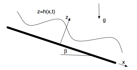
We investigate the stability of free-surface flow on a heated incline. We develop a complete mathematical model for the flow which captures the Marangoni effect and also accounts for changes in the properties of the fluid with temperature. We apply a linear stability analysis to determine the stability of the steady and uniform flow. The associated eigenvalue problem is solved numerically by means of a spectral collocation method. Comparisons with nonlinear simulations are also made and the agreement is good.
Citation: Jean-Paul Pascal, Serge D’Alessio, Syeda Rubaida Zafar. The instability of liquid films with temperature-dependent properties flowing down a heated incline[J]. AIMS Mathematics, 2019, 4(6): 1700-1720. doi: 10.3934/math.2019.6.1700
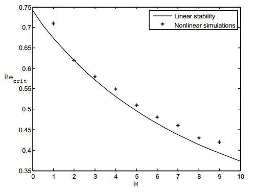
We investigate the stability of free-surface flow on a heated incline. We develop a complete mathematical model for the flow which captures the Marangoni effect and also accounts for changes in the properties of the fluid with temperature. We apply a linear stability analysis to determine the stability of the steady and uniform flow. The associated eigenvalue problem is solved numerically by means of a spectral collocation method. Comparisons with nonlinear simulations are also made and the agreement is good.

| [1] | P. L. Kapitza, Wave flow of thin layers of a viscous fluid: II. Fluid flow in the presence of continuous gas flow and heat transfer, Zh. Eksp. Teor. Fiz., 18 (1948), 19-28. |
| [2] | P. L. Kapitza and S. P. Kapitza, Wave flow of thin layers of a viscous fluid: III. Experimental study of undulatory flow conditions, Zh. Eksp. Teor. Fiz., 19 (1949), 105-120. |
| [3] |
T. B. Benjamin, Wave formation in laminar flow down an inclined plane, J. Fluid Mech., 2 (1957), 554-574. doi: 10.1017/S0022112057000373

|
| [4] |
C.-S. Yih, Stability of liquid flow down an inclined plane, Phys. Fluids, 6 (1963), 321-334. doi: 10.1063/1.1706737
|
| [5] | D. J. Benney, Long waves on liquid films, J. Math. and Phys., 45 (1966), 150-155. |
| [6] | B. Gjevik, Occurrence of Finite-Amplitude Surface Waves on Falling Liquid Films, Phys. Fluids, 13 (1970), 1918-1925. |
| [7] | S. Kalliadasis, E. A. Demekhin, C. Ruyer-Quil, et al. Falling liquid films, Springer-Verlag, London, 2012. |
| [8] |
S. Kalliadasis, E. A. Demekhin, C. Ruyer-Quil, et al. Thermocapillary instability and wave formation on a film flowing down a uniformly heated plane, J. Fluid Mech., 492 (2003), 303-338. doi: 10.1017/S0022112003005809
|
| [9] | C. Ruyer-Quil, B. Scheid, S. Kalliadasis, et al. Thermocapillary long waves in a liquid film flow. part 1. low-dimensional formulation, J. Fluid Mech., 538 (2005), 199-222. |
| [10] | B. Scheid, C. Ruyer-Quil, S. Kalliadasis, et al. Thermocapillary long waves in a liquid film flow. part 2. linear stability and nonlinear waves, J. Fluid Mech., 538 (2005), 223-244. |
| [11] | P. Trevelyan, B. Scheid, C. Ruyer-Quil, et al. Heated falling films, J. Fluid Mech., 592 (2007), 295-334. |
| [12] |
S. Lin, Stability of a liquid flow down a heated inclined plane, Lett. Heat Mass Transfer, 2 (1975), 361-369. doi: 10.1016/0094-4548(75)90002-8
|
| [13] | Y. O. Kabova and V. V. Kuznetsov, Downward flow of a nonisothermal thin liquid film with variable viscosity, J. Appl. Mech. Tech. Phys., 43 (2002), 895-901. |
| [14] | D. A. Goussis and R. A. Kelly, Effects of viscosity on the stability of film flow down heated or cooled inclined surfaces: Long-wavelength analysis, Phys. Fluids, 28 (1985), 3207-3214. |
| [15] | C.-C. Hwang and C.-I. Weng, Non-linear stability analysis of film flow down a heated or cooled inclined plane with viscosity variation, Int. J. Heat Mass Transfer, 31 (1988), 1775-1784. |
| [16] | K. A. Ogden, S. J. D. D'Alessio, J.P. Pascal, Gravity-driven flow over heated, porous, wavy surfaces, Phys. Fluids, 23 (2011), 122102. |
| [17] |
J. P. Pascal, N. Gonputh and S. J. D. D'Alessio, Long-wave instability of flow with temperature dependent fluid properties down a heated incline, Intl J. Eng. Sci., 70 (2013), 73-90. doi: 10.1016/j.ijengsci.2013.05.003
|
| [18] | S. J. D. D'Alessio, C. J. M. P. Seth and J. P. Pascal, The effects of variable fluid properties on thin film stability, Phys. Fluids, 26 (2014), 122105. |
| [19] | M. Chhay, D. Dutykhb, M. Gisclonb, et al. New asymptotic heat transfer model in thin liquid films, Appl. Math. Model., 48 (2017), 844-859. |
| [20] | J. H. Spurk and N. Aksel, Fluid Mechanics, 2nd edition, Springer-Verlag, Berlin, 2008. |
| [21] | C. Ruyer-Quil and P. Manneville, Improved modeling of flows down inclined planes, Eur. Phys. J. B, 15 (2000), 357-369. |
| [22] | C. Ruyer-Quil and P. Manneville, Further accuracy and convergence results on the modeling of flows down inclined planes by weighted-residual approximations, Phys. Fluids, 14 (2002), 170-183. |
| [23] | N. Gonputh, J. P. Pascal and S. J. D. D'Alessio, Inclined flow of a heated fluid film with temperature dependent fluid properties, In: Proceedings of the 2012 International Conference on Scientific Computing, pp. 247-253, CSREA Press, 2012. |
Figures(9)

Jean-Paul Pascal, Serge D’Alessio, Syeda Rubaida Zafar. The instability of liquid films with temperature-dependent properties flowing down a heated incline[J]. AIMS Mathematics, 2019, 4(6): 1700-1720. doi: 10.3934/math.2019.6.1700


 DownLoad: