Contrasting Photo-physiological Responses of the Haptophyte Phaeocystis Antarctica and the Diatom Pseudonitzschia sp. in the Ross Sea (Antarctica)

Abbreviations: BE(s): Bayes estimate(s)\estimator(s); ML: Maximum likelihood; MLE(s): Maximum likelihood estimate(s)\estimator(s); Type-Ⅰ APHCS: Type-Ⅰ adaptive progressive hybrid censoring scheme; Type -Ⅱ APHCS: Type-Ⅱ adaptive progressive hybrid censoring scheme; PCS: Progressive censoring scheme; HPD: Highest posterior density; MC: Monte Carlo; MCMC: Markov Chain Monte Carlo; MH: Metropolis-Hastings; IWD: Inverse Weibull distribution; pdf: Probability density function; cdf: Cumulative density function; hrf: Hazard rate function; sf: Survival function; i.i.d: Independent and identically distributed; IP(s): Informative prior(s); Non-IP: Non-informative prior; CI(s): Confidence interval(s); Asy-CI: Asymptotic confidence interval; St.E: Standard error; MSE: Mean squared-error; AILs: Average interval lengths; CPs: Coverage probabilities

1.   Introduction

Statistical inference for the life products requires placing some units of the product under test to get more information about the life testing experiments to get the complete data, there are many situations where observed data are censored in nature. Different censoring schemes are widely used in practice to make a life testing experiment be more time and cost--effective. Type-Ⅰ and Type-Ⅱ censoring schemes are popular censoring schemes. The experimental duration is set in a Type-Ⅰ censoring scheme, but the number of reported losses is a random variable. Conversely, in a Type-Ⅱ censoring system, the duration of the trial is random while the number of reported losses is constant. However, none of these two censoring schemes any experimental unit can be withdrawn during the experiment. The PCS allows the withdrawal of some experimental units during the experiment. The combination of Type-Ⅰ and Type-Ⅱ censoring schemes is known as a hybrid censoring scheme. Different PCS have been suggested in the literature. The most popular one is the progressive Type-Ⅰ. They are as follows: supposing $n$ identical units are tested; in the traditional Type-Ⅰ censoring system, the experiment continues until a set time has passed $\tau$. In the traditional Type-Ⅱ censoring technique, the experiment is ended after a predefined number of failures $m < n$. Reference ^[1] created the Type-Ⅰ hybrid censoring system, which is a combination of Type-Ⅰ and Type-Ⅱ censoring systems and has been widely utilized in the literature. The life test experiment is ended at a random moment in a mixed censoring strategy. The life test experiment is stopped at a random time ${\tau }^{*} = \mathit{min}\left({y}_{m:m:n}, \tau \right)$ under the hybrid censoring system. Reference ^[2] suggested a novel hybrid censoring strategy to end the ${\tau }^{*} = \mathit{max}\left({y}_{m:m:n}, \tau \right)$. Type-Ⅱ hybrid censoring is the name of this hybrid censoring technique. One of the disadvantages of these approaches is that they prevent the units from being removed from the experiment at any time other than the end. To address this issue, a broader censoring system known as progressive Type-Ⅱ censoring is employed.

The next is a description of the progressive Type-Ⅱ censoring scheme is: during a life-testing experiment, consider an experiment in which $n$ units are placed with $m$ units required to fail. Units ${y}_{1:m:n}, {R}_{1}$ are randomly taken from the remaining $n-1$ surviving units when the first failure occurs. Similarly, when the second failure ${y}_{2:m:n}, {R}_{2}$ occurs, $n-2-{R}_{1}$ units are withdrawn at random from the surviving units, and so on. At the time of the $m-th$ failure ${y}_{m:m:n}$ all remaining $n-m-{R}_{1}-{R}_{2}-...-{R}_{m-1}$units are eliminated when the system fails. Prior the study, the progressively censoring technique ${R}_{1}, {R}_{2}, ..., {R}_{m}$was fixed and set. A Type-Ⅰ PHC system, which is a combination of Type-Ⅱ progressive and hybrid Type-Ⅰ censoring systems, was investigated by references ^[3,4]. In this experiment, $n$identical units are tested using a predetermined progressive filtering technique ${R}_{1}, {R}_{2}, ..., {R}_{m}$, and the experiment is stopped at a random period ${\tau }^{*} = \mathit{min}\left({y}_{m:m:n}, \tau \right)$. If the $m-th$ failure occurs before the time point $\tau$, the experiment ends at that time point if the failure happens before the time point ${y}_{m:m:n}$. Alternatively, assume the $m-th$ failure does not happen before time point $\tau$ and only $J$ failures happen before the time point $\tau$, the experiment concludes at the time point $\tau$ when all the remaining units are removed. Reference ^[5] showed a Type-Ⅱ PHC method, in which the experiment ends at time ${\tau }^{*} = \mathit{max}\left({y}_{m:m:n}, \tau \right)$. Reference ^[6] suggested a Type-Ⅱ APHC system, within which the number of failures $m$ and the related progressive method is provided, but the units are not deleted as the experiment advances time $\tau$. For an all-inclusive survey of the literature on hybrid censoring, see Reference ^[7]. Because of the short time, it takes to create a product, reliability testing has to be undertaken under stern time limitations, which makes failure censored systems out of date in many goods fields. Reference ^[8] presents Type-Ⅰ APHCS that assurances the finish of the lifetime testing experiment at a predetermined time which outcomes in higher estimate competence.

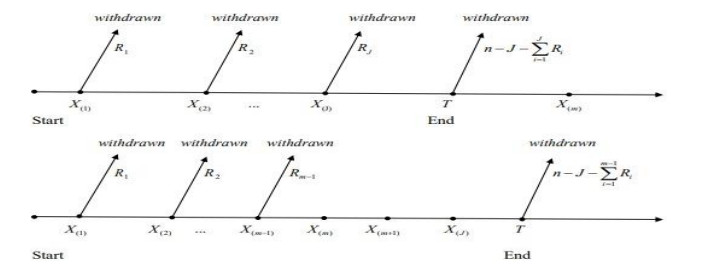
The following is a description of the Type-Ⅰ APHCS (see Reference ^[8]): Assume $n$ similar units are tested using a progressive censoring scheme ${R}_{1}, {R}_{2}, ..., {R}_{m}$, $1\le m\le n$, and the test concludes at a certain point $\tau$, where $\tau \in \left(0, \infty \right)$ and integers ${R}_{i}$'s are prefixed. At the time of the first failure ${y}_{1:m:n}, {R}_{1}$ of the remaining units are randomly removed. Similarly, at the time of the second failure ${y}_{2:m:n}, {R}_{2}$ of the remaining units are randomly removed and so on. Let $J$ denote the number of failures that happen before time $\tau$. If the $m-th$ failure ${y}_{m:m:n}$ happens before time $\tau$ $\left(i.e., {y}_{m:m:n} < \tau \right)$, the process will not stop, but continue on observing failures without any further withdrawals until reach time $\tau$. Then, at time $\tau$ all remaining units ${R}_{J}^{*} = n-J-{\sum }_{i = 1}^{J}{R}_{i}$ are eliminated, and the project is halted. The PCS in this case will become ${R}_{1}, {R}_{2}, ..., {R}_{m}, {R}_{m+1}, ..., {R}_{J}$, where ${R}_{m} = {R}_{m+1} = ... = {R}_{J} = 0$. Otherwise, the process when ${y}_{m:m:n} > \tau$ will have a PCS as ${R}_{1}, {R}_{2}, ..., {R}_{J}$. Type-Ⅰ APHCS is useful when time is the primary consideration in the test and the test must be terminated at a set time irrespective of the amount of failures. Additionally, clarifications may be found in references ^{[8,9,10,11,12,13,14,15,16,17,18]}.

In reliability analysis, an item's failure might be attributed to multiple causes at the same time. These "causes" are competing for control of the experimental unit's failure. This issue is known to as competing risks model in the statistical literature. The data used in the study of competing risks consists of a failure time and the reason of failure. It's possible to presume that the causes of failure are either independent or dependent. For further information about this see ^{[19,20,21,22,23]}.

The primary goal of this research is to examine the competing risk model in the context of a Type-Ⅰ APHCS. We'll also suppose that the lifetimes of the competing hazards have independent IWD. We derive the MLEs, approximate CIs, and two distinct bootstrap CIs; additionally, we used MCMC approaches, to be able to derive BEs for squared error functions and credible intervals using gamma priors.

The following is how the rest of the paper is structured: The IWD is introduced as a failure model in Section Ⅱ. The ML inference of unknown parameters is discussed in Section Ⅲ. Section Ⅳ includes two parametric bootstrap CIs and an approximation CI for unknown parameters. Section Ⅴ investigates the Bayesian estimation approach using the MH algorithm and the gamma distribution as a prior distribution for the unknown parameters. In Section Ⅵ, the theoretical results are illustrated using a simulated study and real data. Finally, Section Ⅶ contains the conclusions. Tables can be found in the appendix.

2.   The IW distribution: as a failure time model Materials and methods

Due to the Weibull distribution's inability to match data with non-monotone and unimodal hazard rate functions, the IWD is a much more suitable model than the Weibull distribution. Depending on the shape parameter's value, the IWD's hrf can decrease or increase. The IWD's pdf, cdf, sf and hrf for single variable $y$, are shown as follows, respectively

and

where $\eta$ and $\varphi$ are the distribution's scale and shape parameters, respectively.

The IWD can be used to show a wide range of data, including the time it takes for an insulating fluid to break down under constant tension, as well as the degradation of mechanical parts like pistons and crankshafts in diesel engines. References ^{[24,25,26,27]} have all done extensive work on the IWD. For further information on the modifications of the IW distribution, read reference ^[28]. Moreover, other articles have looked at IWD under various censoring schemes see references ^{[29,30,31,32,33]}.

3.   ML estimation

In reliability analysis, an item's failure might be attributed to multiple causes at the same time. To failure this experiment unit, these causes are competing for them. Given a lifetime experiment with $n\in N$ identical units, in which the lifetimes are described by i.i.d random variables ${Y}_{1}, {Y}_{2}, ..., {Y}_{n}$. Put the assumption that there are just two causes of failure without losing generality. We have ${Y}_{1} = \mathit{min}\left({Y}_{1i}, {Y}_{2i}\right)$ for $i = \mathrm{1, 2}, ..., n$, where ${Y}_{ki}$, $k = \mathrm{1, 2}$ denotes the $ith$ unit's latent failure time under the $kth$ cause of failure. The latent failure times are assumed to be ${Y}_{1i}$ and ${Y}_{2i}$ are independent, and the pairs $\left({Y}_{1i}, {Y}_{2i}\right)$ are i.i.d. Assume the failure times are distributed according to IWD with different scale and shape parameters $\left({\eta }_{k}, {\varphi }_{k}, k = \mathrm{1, 2}\right)$, with the sf ${\overline F }_{k}$ and hrf ${h}_{k}$ already having form

We have the following observation under Type-Ⅰ APHCS under competing risks data:

where, ${\delta }_{i}$ is the indicator indicating the reason for failure, $J$ is the number of failures prior to time $\tau$, and ${R}_{J}^{*}$ is the number of units residual at the time point $\tau$ with ${R}_{m} = {R}_{m+1}, ..., {R}_{J} = 0$. Let ${\delta }_{i}\in \left(\mathrm{1, 2}\right)$. Here, ${\delta }_{i} = k$, $k = \mathrm{1, 2}$ means the unit $i$ has failed due to cause $k$. Further, we define

Thus, the random variables ${J}_{1} = {\sum }_{i = 1}^{J}{I}_{1}\left({\delta }_{i} = 1\right)$ and ${J}_{2} = {\sum }_{i = 1}^{J}{I}_{2}\left({\delta }_{i} = 2\right)$ show the number of failures due to the first and the second cause of failures, respectively. For a specific censoring scheme, ${R}_{1}, {R}_{2}, ..., {R}_{m-1}, 0, ..., 0, {R}_{J}^{*}$, the observed data's $\left({x}_{1}, {\delta }_{1}\right), ..., \left(\tau, {R}_{J}^{*}\right)$ then, the likelihood function is given by

where ${y}_{i} = {y}_{i:m:n}$ to simplify the notation, ${C}_{J} = {\prod }_{i = 1}^{J}{\gamma }_{i}$ with ${\gamma }_{i} = m-i+1-{\sum }_{i = 1}^{m}{R}_{j}$. Appling the identity${f}_{k} = {h}_{k}{\overline F }_{k}$, The likelihood function can also be written as

In the presence of Type-Ⅰ APHC with competing risks data (6) and from the life time distribution (5), then, ignoring the constant, the likelihood function of the observed data can be written as:

where ${U}_{ki} = \left({e}^{{\eta }_{k}{y}_{i}^{-{\varphi }_{k}}}-1\right)$, ${\psi }_{ki} = \left({\prod }_{i = 1}^{{J}_{k}}{y}_{i}^{-\left({\varphi }_{k}+1\right)}\right)\left[{\prod }_{i = 1}^{{J}_{k}}{U}_{ki}^{-1}\right]$, ${W}_{ki} = \left[1-\mathit{exp}\left(-{\eta }_{k}{y}_{i}^{-{\varphi }_{k}}\right)\right]$, ${y}_{i} = {y}_{\left(i\right)}$, $k = \mathrm{1, 2}$, ${S}_{k} = \left[1-\mathit{exp}\left(-{\eta }_{k}{\tau }^{-{\varphi }_{k}}\right)\right]$ and $L\left(\phi \left|{\underline y }\right.\right) = L\left({\eta }_{1}, {\eta }_{2}, {\varphi }_{1}, {\varphi }_{2}\left|{\underline y }\right.\right)$ for simplicity of notation ${J}_{1} = {\sum }_{i = 1}^{{J}_{1}}I\left({\delta }_{i} = 1\right)$ and ${J}_{2} = {\sum }_{i = 1}^{{J}_{2}}I\left({\delta }_{i} = 2\right)$ describe the number of the failures due to the first and the second cause of the failures, respectively. Using the likelihood function of the natural logarithm $l = \mathit{ln}L\left(\phi \right)$ in Eq (7), we obtain

The first order derivatives of Eq (8) with respect to ${\eta }_{k}, {\varphi }_{k}$, $k = \mathrm{1, 2}$ are given respectively by

where, ${V_{ki}} = y_i^{ - {\varphi _k}}\exp \left({{\eta _k}y_i^{ - {\varphi _k}}} \right)U_{ki}^{ - 1}$, ${Q_{ki}} = y_i^{ - {\varphi _k}}\exp \left({ - {\eta _k}y_i^{ - {\varphi _k}}} \right)W_{ki}^{ - 1}$, ${E_{ki}} = {\tau ^{ - {\beta _k}}}\exp \left({ - {\eta _k}{\tau ^{ - {\varphi _k}}}} \right)S_k^{ - 1}$ and $k = 1, \, 2$. The MLE of ${\eta _k}, \, {\varphi _k}$ and $k = 1, \, 2$ can be obtained by equating the first derivatives in Eqs (9) and (10) to zero. As far as it seems, there is no closed form answer to the system of nonlinear Eqs (9) and (10) in ${\eta _k}, \, {\varphi _k}$ where $k = 1, \, 2$. So, a numerical approach is wanted for competing the MLE of ${\eta _k}, \, {\varphi _k}$ where $k = 1, \, 2$.

The asymptotic variance covariance matrix of the MLEs of $\phi = \left({{\eta _k}, \, {\varphi _k}} \right)$ and $k = 1, \, 2$ are given by the elements that are the negative expectation values of the second derivatives of logarithms of the likelihood functions. Cohen found that by substituting expected values with MLEs, the approximate variance covariance matrix could be calculated—see reference ^[34]. Now, the approximate sample information matrix should now be as follows

where $k = 1, \, 2$ and the elements of $4\times 4$ matrix $I\left(\phi \right)$ can be obtained as follows:

and

Now, we calculate the relative risk rates, ${\pi }_{1}$ and ${\pi }_{2}$ due to case 1 and 2, respectively. The relative risk related to case 1 is calculated as follows:

therefore,

Once ${\pi }_{1}$ is computed, we determine ${\pi }_{2}$ using the relation ${\pi }_{2} = 1-{\pi }_{1}$

We must apply a numerical methodology to solve the integral on the right side of Eq (12) because it has no analytical solution. The MLE of the relative risk rates ${\pi }_{1}$ and ${\pi }_{2}$ can be calculated by substituting the MLE of ${\eta }_{k}, {\varphi }_{k}$ and $k = \mathrm{1, 2}$ in according to the MLE's invariance property Eq (12).

4.   Confidence interval

In this section, Different CIs are suggested. The asymptotic distribution of ${\eta }_{k}, {\varphi }_{k}$, $k = \mathrm{1, 2}$ and two separate bootstrap CIs are used in one.

4.1.   Asy-CI

The asymptotic distribution of the MLEs of the components of the vector of $\phi = \left({\eta }_{k}, {\varphi }_{k}\right)$ and $k = \mathrm{1, 2}$ is being used to derive the approximate CIs for both the parameters. The asymptotic distribution of the MLEs of the parameters is known as

where $I\left(\phi \right)$ is a matrix of Fisher information. When certain regularity constraints are met, the two-sided $100\left(1-\gamma \right)\%$, $0 < \gamma < 1$, asymptotic CIs for the unknown parameters $\phi = \left({\eta }_{k}, {\varphi }_{k}\right)$ and $k = \mathrm{1, 2}$ can be obtained as

where $Var\left(\widehat{\phi }\right)$ is the element of the main diagonal of ${I}^{-1}\left(\widehat{\phi }\right)$ and ${Z}_{\frac{\gamma }{2}}$ is the $100\left(1-\gamma \right)\%$ standard normal percentile.

4.2.   Bootstrap CI

Here, we construct two parametric bootstrap CIs for ${\eta }_{k}, {\varphi }_{k}$, $k = \mathrm{1, 2}$ as

4.2.1.   Percentile bootstrap (Boot-P) CI

1) Calculate the MLE of $\phi = \left({\eta }_{k}, {\varphi }_{k}\right)$ and $k = \mathrm{1, 2}$ under Type-Ⅰ APHCS competing risks data.

2) Generated a bootstrap sample using ${\eta }_{k}, {\varphi }_{k}$, $k = \mathrm{1, 2}$ to obtain the bootstrap estimate of ${\eta }_{k}$ say ${\widehat{\eta }}_{k}^{b}$, ${\varphi }_{k}$ say ${\widehat{\varphi }}_{k}^{b}$ and $k = \mathrm{1, 2}$ using the bootstrap sample.

3) Step (2) is repeated B times to have $\left({\eta }_{k}^{b\left(1\right)}, {\eta }_{k}^{b\left(2\right)}, ..., {\eta }_{k}^{b\left(B\right)}\right)$ and $\left({\varphi }_{k}^{b\left(1\right)}, {\varphi }_{k}^{b\left(2\right)}, ..., {\varphi }_{k}^{b\left(B\right)}\right)$.

4) By arranging $\left({\eta }_{k}^{b\left(1\right)}, {\eta }_{k}^{b\left(2\right)}, ..., {\eta }_{k}^{b\left(B\right)}\right)$, $\left({\varphi }_{k}^{b\left(1\right)}, {\varphi }_{k}^{b\left(2\right)}, ..., {\varphi }_{k}^{b\left(B\right)}\right)$ in ascending order as $\left({\eta }_{k}^{b\left[1\right]}, {\eta }_{k}^{b\left[2\right]}, ..., {\eta }_{k}^{b\left[B\right]}\right)$ and $\left({\varphi }_{k}^{b\left[1\right]}, {\varphi }_{k}^{b\left[2\right]}, ..., {\varphi }_{k}^{b\left[B\right]}\right)$.

A two side $100\left(1-\gamma \right)\%$ percentile bootstrap CI for ${\eta }_{k}, {\varphi }_{k}$ and $k = \mathrm{1, 2}$ is given by $\left\{{\widehat{\eta }}_{k}^{b\left[B\frac{\gamma }{2}\right]}, {\widehat{\eta }}_{k}^{b\left[B\right(1-\frac{\gamma }{2}\left)\right]}\right\}$ and $\left({\widehat{\varphi }}_{k}^{b\left[B\frac{\gamma }{2}\right]}, {\widehat{\varphi }}_{k}^{b\left[B\right(1-\frac{\gamma }{2}\left)\right]}\right)$.

4.2.2.   Bootstrap-t CI

1) The same as in Boot-p steps (1-2).

2) Calculate the t-statistic of $\phi = \left({\eta }_{k}, {\varphi }_{k}\right)$ and $k = \mathrm{1, 2}$ as $T = \frac{\left({\widehat{\phi }}_{k}^{b}-{\widehat{\phi }}_{k}\right)}{\sqrt{Var\left({\widehat{\phi }}_{k}^{b}\right)}}$ where $Var\left({\hat \varphi _k^b} \right)$ is asymptotic variances of ${\widehat{\phi }}_{k}^{b}$ and it can be obtained using the Fisher information matrix.

3) Step 2–3 are repeated $B$ times and obtain ${T}^{\left(1\right)}, {T}^{\left(2\right)}, ..., {T}^{\left(B\right)}$.

4) By arranging ${T}^{\left(1\right)}, {T}^{\left(2\right)}, ..., {T}^{\left(B\right)}$ in ascending order as ${T}^{\left[1\right]}, {T}^{\left[2\right]}, ..., {T}^{\left[B\right]}$.

5) A two side $100\left(1-\gamma \right)\%$ percentile bootstrap-t CI for ${\eta }_{k}, {\varphi }_{k}$ and $k = \mathrm{1, 2}$ is given by

5.   Bayesian estimation

In this section, based on competing risks data, the BE utilizing square error loss functions are obtain based on a Type-Ⅰ APHCS under the assumption independently distributed with gamma prior distribution with known parameters ${\eta }_{k}, {\varphi }_{k}$ where $k = \mathrm{1, 2}$ of the IWD as

and

where the hyper-parameters ${a}_{k}, {b}_{k}, {c}_{k}, {d}_{k}$ and $k = \mathrm{1, 2}$ are chosen based on prior knowledge of the unknown parameters. Then we can write the jointly prior densities of ${\eta }_{k}, {\varphi }_{k}$ and $k = \mathrm{1, 2}$ as

when the IPs are taken into account, the hyper-parameter elicitation will be chosen. The MLEs of ${\eta }_{k}, {\varphi }_{k}$ and $k = \mathrm{1, 2}$ will be used to generate these IPs. Equal the mean and variance of $\left({\widehat{\eta }}_{k}^{q}, {\widehat{\varphi }}_{k}^{q}\right)$ with the mean and variance of the priors under consideration (Gamma priors), where $k = \mathrm{1, 2}$ and $q = \mathrm{1, 2}, ..., N$, here $N$ is really the number of samples from the IWD that are available. Thus, when the mean and variance of ${\widehat{\eta }}_{k}^{q}$ and ${\widehat{\varphi }}_{k}^{q}$ are equal to the mean and variance of gamma priors, one can obtain (see reference ^[35])

The estimated hyper-parameters now have the following forms after solving the about equations

For the observed data $\mathit{y}$ acquired from a life test experiment's Type-Ⅰ APHCS with two independent IW $\left({\eta }_{1}, {\varphi }_{1}\right)$ and IW $\left({\eta }_{2}, {\varphi }_{2}\right)$ and given the likelihood function in Eq (7) and prior distribution in Eq (13). The corresponding posterior density of $\phi = \left({\eta }_{k}, {\varphi }_{k}\right)$ and $k = \mathrm{1, 2}$ is given by

The posterior density function is given by

where ${\omega }_{ki}\left(\phi \right) = {\psi }_{ki}\left[{\prod }_{i = 1}^{J}{\left({W}_{1i}{W}_{2i}\right)}^{\left(1+{R}_{i}\right)}\right]{\left[{S}_{1}{S}_{2}\right]}^{{R}_{J}^{*}}$.

The conditional posterior densities of $\phi = \left({\eta }_{k}, {\varphi }_{k}\right)$ and $k = \mathrm{1, 2}$ are as follows

As a result, we use the MH method to generate according to the above distribution see reference ^[36]. Readers can consult reference ^[37] for more information on how to implement the MH algorithm. We started also with MLEs to drive the Gibbs sampler algorithm. We then choose samples from different complete conditionals in the runs, using very latest readings of all other conditioning variables, unless a consistent pattern of convergence was seen. While, the BEs of any function say $g\left({\eta }_{1}, {\varphi }_{1}, {\eta }_{2}, {\varphi }_{2}\right)$ based on Type-Ⅰ APHCS with competing risks under square error loss functions; denoted by $\widetilde{g}\left({\eta }_{k}, {\varphi }_{k}\right)$ can be studied through the following equation as

Closed form of equations cannot be used for obtaining the ratio of the four integrals demonstrated in Eq (15). Therefore, we recommend the MCMC method to reach an approximated value of the BEs of ${\eta }_{k}, {\varphi }_{k}, k = \mathrm{1, 2}$. Using MH algorithm, this technique can generate a posterior sample. Several authors state that MCMC is a computer-based sampling technique that enables a user to indicate and define a distribution regardless of its mathematical characteristics obtained by random sampling values—see reference ^[38]. Working with posterior distributions, it is more profitable to use MCMC rather than using analytic examination which is very hard to work with. The MCMC makes it easy for the user to reach rough values of posterior distributions which is cannot be easily measured using a computer (like posteriors means and its random samples). Using the MCMC technique, samples are:

1) Start with a wild preliminary guess: a single value that could be derived from the distribution.

2) Using this preliminary assumption, generate a series of new samples. Two steps are created as a result of each new sample:

● Proposal: the most recent sample is disturbed with a small random perturbation to provide a proposal for the new sample.

● Acceptance: a novel suggestion will be either approved as a new sample or rejected (in which case the old sample is retained). There are several methods for introducing random noise into the system to generate ideas, as well as numerous methods for approving and refusing them, such as Gibbs sampling and the MH algorithm.

5.1.   MH algorithm

A proposing distribution and also a preliminary value of $\phi = \left({\eta }_{k}, {\varphi }_{k}\right)$ and $k = \mathrm{1, 2}$ must always be defined in order to conduct the MH method for the IWD. A multivariate normal distribution can be used to represent the proposal distribution as

where ${S}_{\left\{{\lambda }_{k}, {\beta }_{k}\right\}}$ represents the variance-covariance matrix, it is possible to acquire negative observations, which is undesirable. For starting values, the MLE may be used as $\phi = \left({\eta }_{k}, {\varphi }_{k}\right)$ and $k = 1, 2$, that is $\left\{{\eta }_{k}^{\left(0\right)}, {\varphi }_{k}^{\left(0\right)}\right\} = \left\{{\widehat{\eta }}_{k}, {\widehat{\varphi }}_{k}\right\}$. The selection of ${S}_{\left\{{\eta }_{k}, {\varphi }_{k}\right\}}$ is considered to be the asymptotic variance-covariance matrix ${I}^{-1}\left\{{\widehat{\eta }}_{k}, {\widehat{\varphi }}_{k}\right\}$, where $I\left\{.\right\}$ is an abbreviation for Fisher information matrix. It is worth noting that the choice of ${S}_{\left\{{\eta }_{k}, {\varphi }_{k}\right\}}$ is a critical issue in the MH algorithm, as the acceptance is dependent on it. The steps of the MH method for drawing a sample from the posterior density Eq (14) are as follows

Step 1. Set initial value of $\phi$ as ${\phi }^{\left(0\right)} = \left\{{\widehat{\eta }}_{1}, {\widehat{\varphi }}_{1}, {\widehat{\eta }}_{2}, {\widehat{\varphi }}_{2}\right\}$.

Step 2. For $i = \mathrm{1, 2}, ..., M$ the following steps are repeating:

a) Set $\phi = {\phi }^{(i-1)}$.

b) Generate a new candidate parameter value $\varsigma$ from ${N}_{4}\left(\mathit{ln}\phi, {S}_{\phi }\right)$.

c) Set ${\phi }^{\mathrm{\text{'}}} = \mathit{exp}\left(\varsigma \right)$.

d) Calculate $\zeta = \frac{\pi \left({\phi }^{\mathrm{\text{'}}}\left|y\right.\right)}{\pi \left(\phi \left|y\right.\right)}$, where $\pi \left(.\right)$ is the posterior density in Eq (14).

e) Generate a sample $u$ from the uniform distribution $U\left(\mathrm{0, 1}\right)$.

f) Accept or reject the new candidate ${\phi }^{\mathrm{\text{'}}}$

Finally, part of the initial samples taken from the posterior density's random samples of size $M$ can be discarded (burn-in), and the surviving samples may be utilized to compute BEs. More specifically, Eq (14) can be calculated as

where ${l}_{\zeta }$ defines the number of burn-in samples.

5.2.   HPD

In this subsection, for $k = \mathrm{1, 2}$, one can unutilized method of reference ^[39] to construct the HPD credible intervals for ${\eta }_{k}$ and ${\varphi }_{k}$ of the IWD under Type-Ⅰ APHCS with competing risks data using the samples drawn from suggested MH algorithm in the previous subsection. Let ${\eta }_{k}^{\gamma }$ and ${\varphi }_{k}^{\gamma }$ be the ${\gamma }^{th}$ quantile of ${\eta }_{k}$ and ${\varphi }_{k}$, respectively, that is,

where $0 < \gamma < 1$ and ${\mathit{\Pi}} \left(.\right)$ is the posterior distribution function of the unknown parameters ${\eta }_{k}, {\varphi }_{k}$ and $k = \mathrm{1, 2}$. Notice that for a given ${\eta }_{k}^{*}, {\varphi }_{k}^{*}$ and $k = \mathrm{1, 2}$, a simulation consistent estimator of $\pi \left({\eta }_{k}, {\varphi }_{k}\left|y\right.\right)$ can be evaluated as

Here ${I}_{\left\{{\eta }_{k}, {\varphi }_{k}\right\}\le \left({\eta }_{k}^{*}, {\varphi }_{k}^{*}\right)}$ is the indicator function. Then the corresponding estimate is calculated as follows:

where ${w}_{s} = \frac{1}{M-{l}_{\zeta }}$ and $\left\{{\eta }_{k\left(s\right)}, {\varphi }_{k\left(s\right)}\right\}$ are the ordered values of $\left\{{\eta }_{ks}, {\varphi }_{ks}\right\}$. Now, for $i = {l}_{\zeta }, ..., M, \left\{{\eta }_{k}^{\left(\gamma \right)}, {\varphi }_{k}^{\left(\gamma \right)}\right\}$ can be convergent by

Now to obtain a $100\left(1-\gamma \right)\%$ HPD credible interval for ${\eta }_{k}, {\varphi }_{k}$ and $k = \mathrm{1, 2}$, let

for $s = {l}_{\zeta }, ..., \left[\gamma M\right]$. Then choose $HP{D}_{{s}^{*}}$ among all the $HP{D}_{s}$'s such that it has the smallest width.

6.   Simulation study and data analysis

The purpose of this section is to compare the results of the various estimation methods presented in the previous parts. A MC analysis is used to evaluate the statistical behaviors of the estimators within Type-Ⅰ APHCS under competing risks mode, as well as to check the behavior of the suggested approaches. A real data collection is also evaluated for demonstration. For calculations, the R statistical programming language will be utilized. In addition, the bbmle and HDInterval packages in R can be used to compute MLEs and HPD intervals.

6.1.   Simulation study

To compare the performance of suggested MC estimation methods, a simulation study is used. The MC simulation is carried out utilizing two estimate methods: ML and Bayesian estimations. With the following assumptions, 1000 data sets of IWD competing risks model under Type-Ⅰ PHCS are generated for MLEs.

1) Assume the parameters of the IWD in the following options: $\left({\eta }_{1}, {\varphi }_{1}, {\eta }_{2}, {\varphi }_{2}\right) = \left(0.5, 1.5, 0.75, 2\right)$.

2) For each cause of failure, the sample sizes are $n = \mathrm{50,100,200}$ and the number of failures observed $m = 20, 40, 60$.

3) Number of re-samplings for bootstrap CI is 1000.

4) Censoring times for Type-Ⅰ APHCS are assumed as: $\tau = 1, 1.5, 2$.

5) Removed items ${R}_{j}$ are assumed to as follows:

Scheme Ⅰ: ${R}_{1} = n-m$ and ${R}_{2} = ... = {R}_{m} = 0$.

Scheme Ⅱ: ${R}_{1} = ... = {R}_{\frac{m}{2}} = 0$, ${R}_{\left(\frac{m}{2}+1\right)} = n-m$ and ${R}_{\left(\frac{m}{2}+2\right)} = ... = {R}_{m} = 0$.

Scheme Ⅲ: ${R}_{1} = ... = {R}_{m-1} = 0$ and ${R}_{m} = n-m$.

MLEs and related to 95% asymptotic CI and two types of bootstrap CI are calculate based on the generated data. Note that the preliminary guess values are regarded as the same as the true parameter values whilst gaining MLEs. Also, we used the MH algorithm to computed BEs by the IP and Non-IP. Thus:

● For IP, we assume that the hyper-parameter values as ${a}_{1} = {b}_{1} = 0.5$, ${c}_{1} = {d}_{1} = 1.5$, ${a}_{2} = {b}_{2} = 0.75$, ${c}_{2} = {d}_{2} = 2$.

● For Non-IP, we assume that the hyper-parameter values are ${a}_{1} = {b}_{1} = {c}_{1} = {d}_{1} = {a}_{2} = {b}_{2} = {c}_{2} = {d}_{2} = 0,$ hence the joint prior density is defined as $\pi \left({\eta }_{1}, {\varphi }_{1}, {\eta }_{2}, {\varphi }_{2}\right) = \frac{1}{{\eta }_{1}\times {\varphi }_{1}\times {\eta }_{2}\times {\varphi }_{2}}$.

These values, referred to as hyper-parameters, are then used to produce the desired estimations. When the MH method is used, the MLEs are used as preliminary guess estimates, together with the associated variance-covariance matrix ${S}_{\phi }$ of $\left[\mathit{ln}\left({\eta }_{1}\right), \mathit{ln}\left({\varphi }_{1}\right), \mathit{ln}\left({\eta }_{2}\right), \mathit{ln}\left({\varphi }_{2}\right)\right]$ which can be obtained using delta method (see reference ^[40]). Lastly, 1200 burn-in samples are removed from the total 6000 samples obtained from the posterior density and subsequent BE and HPD interval estimations.

Tables 1–3 are showing all of the average bias estimates and related MSEs for both methods. Furthermore, the corresponding AILs and CPs are presented in Tables 4–6 for all of the suggested CIs, namely; Asy-CI, bootstrap (Boot-P and Boot-T) CI, and HPD interval.

From tabulated values, it can be noted that, higher values of $n$ lead to decreasing in MSE depending on the MSEs. With increasing in $n$ and $m$, the average bias of the estimated values is increasing for the parameters ${\eta }_{1}$, ${\varphi }_{2}$ and decreasing for the parameters ${\eta }_{2}$ and ${\varphi }_{1}$. Also, the average bias of the estimated values of the parameters, ${\varphi }_{1}$ and ${\varphi }_{2}$, of the MLEs is fewer than the BEs (IP and Non-IP) and for parameters, ${\eta }_{1}$ and ${\eta }_{2}$, of the MLEs are higher than the BEs. Furthermore, The BEs under IP for the parameters are better than BEs under Non-IP for the same parameters. Comparing the results in Tables 4–6, we noted that the HPD intervals under IP perform better than the HPD intervals under Non-IP based on minimum confidence/credible intervals lengths. Also, The AILs of the Asy-CI of the MLEs have the shortest length among the suggested CIs, the AIL decreases in general as $n$ and $m$ increase. In addition, according to the CPs, the MLEs technique has the highest CP among the suggested CPs. Our simulation study's major conclusion is that as the number of steps in a progressive Type-Ⅰ censoring scheme rises over time, the average bias of the estimates and MSEs diminish.

6.2.   Real data

A real-world data set is used to illustrate the concept and to determine the statistical measures of the MLEs and BEs for IWD under a variety of Type-Ⅰ APHCS using a competing risks model.

The set of data beneath was first examined by reference ^[41] and was subsequently examined by reference ^[21]. The finding was obtained in a laboratory experiment in which male mice were administered a 300-roentgen radiation dosage between the ages of 35 and 42 days (5–6 weeks). For each mouse, the cause of death was identified as reticulum cell sarcoma as 1 (^*) and other reasons of death as cause 2 (^**), there were $n = 77$ observations remain in the analysis registered below: 40^**, 42^**, 51^**, 62^**, 163^**, 179^**, 206^**, 222^**, 228^**, 249^**, 252^**, 282^**, 317^*, 318^*, 324^**, 333^**, 341^**, 366^**, 385^**, 399^*, 407^**, 420^**, 431^**, 441^**, 461^**, 462^**, 482^**, 495^*, 517^**, 517^**, 524^**, 525^*, 536^*, 549^*, 552^*, 554^*, 557^*, 558^*, 564^**, 567^**, 571^*, 586^*, 586^**, 594^*, 596^*, 605^*, 612^*, 619^**, 620^**, 621^*, 621^**, 622^**, 628^*, 631^*, 636^*, 643^*, 647^*, 647^**, 648^*, 649^*, 651^**, 661^*, 663^*, 666^*, 670^*, 686^**, 695^*, 697^*, 700^*, 705^*, 712^*, 713^*, 738^*, 748^*, 753^*, 761^**, 763^**.

From data original, one can create, e.g., five Type-Ⅰ APHC samples with a number of stages $m = 30$ at time censoring $\tau = 400$ and removed items ${R}_{j}$ (randomly from the surviving items) are assumed to as follows:

Scheme Ⅰ: ${R}_{1} = n-m$ and ${R}_{2} = ... = {R}_{m} = 0$.

Scheme Ⅱ: ${R}_{1} = ... = {R}_{\frac{m}{2}} = 0$, ${R}_{\left(\frac{m}{2}+1\right)} = n-m$ and ${R}_{\left(\frac{m}{2}+2\right)} = ... = {R}_{m} = 0$.

Scheme Ⅲ: ${R}_{1} = ... = {R}_{m-1} = 0$ and ${R}_{m} = n-m$.

Scheme Ⅳ: $\tau = 800$, ${R}_{1} = n-m$ and ${R}_{2} = ... = {R}_{m} = 03$.

Scheme Ⅴ: $\tau = 800$ and ${R}_{1} = {R}_{2} = ... = {R}_{m} = 0$.

Note that: Scheme Ⅳ can be considered as a progressive Type-Ⅱ censoring scheme, a special case of Type-Ⅰ APHCS. Also, complete sampling can be considered as a special case of Type-Ⅰ APHCS in Scheme Ⅴ when ${R}_{1} = {R}_{2} = ... = {R}_{m} = 0$.

The MLEs of ${\eta }_{1}, {\varphi }_{1}, {\eta }_{2}$ and ${\varphi }_{2}$, as well as their related asymptotic CI, two types of bootstrap CI estimates, and AIL for Type-Ⅰ APHC samples under competing risks model with two independent causes of failures as in the given real data set, are shown in Table 7. In addition, BEs were calculated using the MH method with the Non-IP. It is indicated that, while generating samples from the posterior distribution utilizing the MH algorithm, preliminary values of $\left({\eta }_{k}, {\varphi }_{k}\right)$ are considered as $\left({\eta }_{k}^{\left(0\right)}, {\varphi }_{k}^{\left(0\right)}\right) = \left({\widehat{\eta }}_{k}, {\widehat{\varphi }}_{k}\right)$, $k = \mathrm{1, 2}$ and $\left({\widehat{\eta }}_{k}, {\widehat{\varphi }}_{k}\right)$ are the MLEs of the parameters$\left({\eta }_{k}, {\varphi }_{k}\right)$. BEs and HPD intervals were then obtained from the remaining 2000 burn-in samples from the posterior density. Each censoring scheme's relative risk will be calculated.

The convergence of MCMC estimation in case of scheme Ⅱ of Type-Ⅰ APHCS for the cause 1, i.e., $\left({\eta }_{1}, {\varphi }_{1}\right)$ can be showed in Figure 2 and for the cause 2, i.e., $\left({\eta }_{2}, {\varphi }_{2}\right)$ can be showed in Figure 3.

7.   Conclusions

A competing risks model under Type-Ⅰ APHCS technique was explained in this paper. When a fixed number of failure causes are known. Assuming that the lifetime distributions are IWD. The MLEs have been generated, and different CIs for the parameters of the IWD has been suggested using asymptotic distributions and bootstrap CIs. Also provided are the HPD intervals. Different sample sizes and censoring schemes are used to differentiate between different estimators and CIs in a simulation study. Also, using the MH method, BEs based on squared error loss function under the assumption of independent gamma priors were produced. In terms of minimum MSEs, the simulation results show that BEs, provide the importance sampling technique better than the other estimates. It's also important to note that among the various CIs, the HPD intervals have the shortest lengths. We studied two real data sets to illustrate how the suggested estimators perform in real. According to the real data analysis, the Type-Ⅰ APHCS technique appears to be highly effective when the experimenter's primary concern is time and it is not required to terminate the experiment at a predefined number of failures. Finally, future research may be interested in locating a real-life Type-Ⅰ APHCS situation and using the suggested approaches presented here, as well as comparing the results to other censoring schemes.

Acknowledgments

This study was funded by Taif University Researchers Supporting Project number (TURSP-2020/279), Taif University, Taif, Saudi Arabia.

Conflict of Interest

The authors have no conflict of interest regarding publishing this paper.