


Figure 1.
The graph
Citation: Charalambos Chasos, George Karagiorgis, Chris Christodoulou. Technical and Feasibility Analysis of Gasoline and Natural Gas Fuelled Vehicles[J]. AIMS Energy, 2014, 2(1): 71-88. doi: 10.3934/energy.2014.1.71
| [1] | Ceyu Lei, Xiaoling Han, Weiming Wang . Bifurcation analysis and chaos control of a discrete-time prey-predator model with fear factor. Mathematical Biosciences and Engineering, 2022, 19(7): 6659-6679. doi: 10.3934/mbe.2022313 |
| [2] | A. Q. Khan, M. Tasneem, M. B. Almatrafi . Discrete-time COVID-19 epidemic model with bifurcation and control. Mathematical Biosciences and Engineering, 2022, 19(2): 1944-1969. doi: 10.3934/mbe.2022092 |
| [3] | Yangyang Li, Fengxue Zhang, Xianglai Zhuo . Flip bifurcation of a discrete predator-prey model with modified Leslie-Gower and Holling-type III schemes. Mathematical Biosciences and Engineering, 2020, 17(3): 2003-2015. doi: 10.3934/mbe.2020106 |
| [4] | Xiaoling Han, Xiongxiong Du . Dynamics study of nonlinear discrete predator-prey system with Michaelis-Menten type harvesting. Mathematical Biosciences and Engineering, 2023, 20(9): 16939-16961. doi: 10.3934/mbe.2023755 |
| [5] | Yajie Sun, Ming Zhao, Yunfei Du . Multiple bifurcations of a discrete modified Leslie-Gower predator-prey model. Mathematical Biosciences and Engineering, 2023, 20(12): 20437-20467. doi: 10.3934/mbe.2023904 |
| [6] | Abdul Qadeer Khan, Azhar Zafar Kiyani, Imtiaz Ahmad . Bifurcations and hybrid control in a 3×3 discrete-time predator-prey model. Mathematical Biosciences and Engineering, 2020, 17(6): 6963-6992. doi: 10.3934/mbe.2020360 |
| [7] | Ming Chen, Menglin Gong, Jimin Zhang, Lale Asik . Comparison of dynamic behavior between continuous- and discrete-time models of intraguild predation. Mathematical Biosciences and Engineering, 2023, 20(7): 12750-12771. doi: 10.3934/mbe.2023569 |
| [8] | Rajalakshmi Manoharan, Reenu Rani, Ali Moussaoui . Predator-prey dynamics with refuge, alternate food, and harvesting strategies in a patchy habitat. Mathematical Biosciences and Engineering, 2025, 22(4): 810-845. doi: 10.3934/mbe.2025029 |
| [9] | Parvaiz Ahmad Naik, Muhammad Amer, Rizwan Ahmed, Sania Qureshi, Zhengxin Huang . Stability and bifurcation analysis of a discrete predator-prey system of Ricker type with refuge effect. Mathematical Biosciences and Engineering, 2024, 21(3): 4554-4586. doi: 10.3934/mbe.2024201 |
| [10] | Minjuan Gao, Lijuan Chen, Fengde Chen . Dynamical analysis of a discrete two-patch model with the Allee effect and nonlinear dispersal. Mathematical Biosciences and Engineering, 2024, 21(4): 5499-5520. doi: 10.3934/mbe.2024242 |
A Reinforced material is a composite building material consisting of two or more materials with different properties. The main objective of studies of reinforced materials is the prediction of their macroscopic behavior from the properties of their individual components as well as from their microstructural characteristics.
The theory of ideal fiber-reinforced composites was initiated by Adkins and Rivlin [4] who studied the deformation of a structure reinforced with thin, flexible and inextensible cords, which lie parallel and close together in smooth surfaces. This theory was further developed by the authors in [44], [1], [2], [3], [45].
The homogenization of elastic materials reinforced with highly contrasted inclusions has been considered by several authors in the two last decades (see for instance [6], [10], [17], [21], [18], and the references therein). The main result is that the materials obtained by the homogenization procedure have new elastic properties.
The homogenization of structures reinforced with fractal inclusions has been considered by various authors, among which [39], [31], [40], [41], [12], [42], [13], and [14]. Lancia, Mosco and Vivaldi studied in [31] the homogenization of transmission problems across highly conductive layers of iterated fractal curves. In [40], Mosco and Vivaldi dealt with the asymptotic behavior of a two-dimensional membrane reinforced with thin polygonal strips of large conductivity surrounding a pre-fractal curve obtained after
The homogenization of insulating fractal surfaces of Koch type approximated by three-dimensional insulating layers has been performed by Capitanelli et al. in [12], [13], and [14]. Due to the physical characteristics of the inclusions, singular energy forms containing fractal energies are obtained in these articles as the limit of non-singular full-dimensional energies. On the other hand, the effective properties of elastic materials fixed on rigid thin self-similar micro-inclusions disposed along two and three dimensional Sierpinski carpet fractals have been recently obtained in [20].
In the present work, we consider the deformation of a three-dimensional elastic material reinforced with highly contrasted thin vertical strips constructed on horizontal iterated Sierpinski gasket curves. Our main purpose is to describe the macroscopic behavior of the composite as the width of the strips tends to zero, their material coefficients tend to infinity, and the sequence of the iterated Sierpinski gasket curves converges to the Sierpinski gasket in the Hausdorff metric.
The asymptotic analysis of problems of this kind was previousely studied in [11], [26], [9], and [5], where the authors considered media comprising low dimensional thin inclusions or thin layers of higher conductivity or higher rigidity. The limit problems consist in second order transmission problems. Problems involving thin highly conductive fractal inclusions have been addressed in a series of papers (see for instance [39], [31], [12], [14], and [19]). The obtained mathematical models are elliptic or parabolic boundary value problems involving transmission conditions of order two on the interfaces. The homogenization of three-dimensional elastic materials reinforced by highly rigid fibers with variable cross-section, which may have fractal geometry, has been carried out in [21]. The authors showed that the geometrical changes induced by the oscillations along the fiber-cross-sections can provide jumps of displacement fields or stress fields on interfaces, including fractal ones, due to local concentrations of elastic rigidities. Note that the numerical approximation of second order transmission problems across iterated fractal interfaces has been considered in some few papers among which [32] and [15].
Let us first consider the points
| $ Vh+1=Vh∪(2−hA2+Vh)∪(2−hA3+Vh). $ | (1) |
Let us set
| $ {{\mathcal V}_\infty } = \mathop \cup \limits_{h \in \mathbb{N} } {{\mathcal V}_h}{{.}} $ | (2) |
The Sierpinski gasket, which is denoted here by
| $ Σ=¯V∞. $ | (3) |
We define the graph
The edges which belong to
Let
| $ Σ∩∂ω=V0. $ | (4) |
Let
| $ limh→∞εh2h=0. $ | (5) |
We define
| $ Tkh=(ω∩Skh)×(−εh,εh) $ | (6) |
and set
| $ {T_h} = \mathop \cup \limits_{k \in {I_h}} T_h^{,k}{\rm{,}}$ | (7) |
where
| $ |Th|=εh3h+12h. $ | (8) |
Let
| $ σij(u)=λemm(u)δij+2μeij(u) ; i,j=1,2,3, $ | (9) |
where the summation convention with respect to repeated indices has been used and will be used in the sequel, and
| $ σhij(u)=λhemm(u)δij+2μheij(u) ; i,j=1,2,3, $ |
with
| $ λh=ηhλ0 and μh=ηhμ0, $ | (10) |
where
| $ ηh=1εh(56)h. $ | (11) |
The special scaling (10) and (11) of the Lamé -coefficients depend on the structural constants of
We suppose that a perfect adhesion occurs between
| $ Fh(u)={∫Ω∖Thσij(u)eij(u)dx+∫Thσhij(u)eij(u)dsdx3 if u∈H10(Ω,R3)∩H1(Th,R3),+∞ otherwise, $ | (12) |
where
| $ minu∈L2(Ω,R3)∩L2(Th,R3){Fh(u)−2∫Ωf.udx}. $ | (13) |
We use
| $ γ=limh→∞(−3h+12hlnεh), $ | (14) |
which is associated with the size of the boundary layers taking place in the neighbourhoods of the fractal strips, we prove that if
| $ F∞(u,v)={∫Ωσij(u)eij(u)dx+μ0∫ΣdLΣ(¯v)+πμγHd(Σ)(ln2)2∫ΣA(s)(u−v).(u−v)dHd(s) if (u,v)∈H10(Ω,R3)×DΣ,E×L2Hd(Σ),+∞ otherwise, $ | (15) |
where
| $ d=ln3/ln2, $ | (16) |
| $ A(s)={Diag(1,2(1+κ),2(1+κ)) if n(s)=±(0,1),(7+κ4(1+κ)√3(κ−1)4(1+κ)0√3(κ−1)4(1+κ)3κ+54(1+κ)0002(1+κ))if n(s)=±(−√32,12),(7+κ4(1+κ)√3(1−κ)4(1+κ)0√3(1−κ)4(1+κ)3κ+54(1+κ)0002(1+κ))if n(s)=±(√32,12), $ | (17) |
where
The effective energy (15) contains new degrees of freedom implying nonlocal effects associated with thin boundary layer phenomena taking place near the fractal strips and a singular energy term supported on the Sierpinski gasket
| $ { [σα3|x3=0]Σ=πμγHd(Σ)(ln2)2Aαβ(s)(Uβ−Vβ)Hd on Σ,πμγ(ln2)2Aαβ(s)(Uβ−Vβ)=−μ0ΔΣVα in Σ; α,β=1,2, $ | (18) |
where
| $ [σα3|x3=0]Σ=σα3|Σ×{0+}−σα3|Σ×{0−}; α=1,2, $ | (19) |
is the jump of
The graph

The network
If
| $ F∞(u)={∫Ωσij(u)eij(u)dx+μ0∫ΣdLΣ(¯u) if u∈H10(Ω,R3)∩(DΣ,E×L2Hd(Σ)), +∞ otherwise. $ | (20) |
If
| $ F0(u)={∫Ωσij(u)eij(u)dx if u∈H10(Ω,R3), +∞ otherwise. $ | (21) |
The paper is organized as follows: in Section 2 we introduce the energy form and the notion of a measure-valued local energy on the Sierpinski gasket
In this Section we introduce the energy form and the notion of a measure-valued local energy (or Lagrangian) on the Sierpinski gasket. For the definition and properties of Dirichlet forms and measure energies we refer to [24], [35], and [37].
For any function
| $ EhΣ(w)=(53)h∑p,q∈Vh|p−q|=2−h|w(p)−w(q)|2. $ | (22) |
Let us define the energy
| $ EΣ(z)=limh→∞EhΣ(z), $ | (23) |
with domain
| $ D={z∈C(Σ,R2):EΣ(z)<∞}, $ | (24) |
where
| $ DE=¯D‖.‖DE, $ | (25) |
where
| $ ‖z‖DE={EΣ(z)+‖z‖2L2Hd(Σ,R2)}1/2. $ | (26) |
The space
| $ DΣ,E={z∈DE:z(A1)=z(A2)=z(A3)=0}. $ | (27) |
We denote
| $ EΣ(w,z)=12(EΣ(w+z)−EΣ(w)−EΣ(z)), ∀w,z∈DΣ,E. $ | (28) |
One can see that
| $ EΣ(w,z)=limh→∞EhΣ(w,z), $ | (29) |
where
| $ EhΣ(w,z)=(53)h∑p,q∈Vh|p−q|=2−h(w(p)−w(q)).(z(p)−z(q)). $ | (30) |
The form
1. (local property)
2. (regularity)
The second property implies that
Now, applying [29,Chap. 6], we have the following result:
Lemma 2.1. There exists a unique self-adjoint operator
| $ DΔΣ={w=(w1w2)∈L2Hd(Σ,R2):ΔΣw=(ΔΣw1ΔΣw2)∈L2Hd(Σ,R2)}⊂DΣ,E $ |
dense in
| $ EΣ(w,z)=−∫Σ(ΔΣw).zdHdHd(Σ). $ |
Let us consider the sequence
| $ νh=1Card(Vh)∑p∈Vhδp, $ | (31) |
where
Lemma 2.2. The sequence
| $ \begin{equation*} \nu = \boldsymbol{1}_{\Sigma }\left( s\right) \dfrac{d\mathcal{H}^{d}\left( s\right) }{\mathcal{H}^{d}\left( \Sigma \right) }\mathit{\text{,}} \end{equation*} $ |
where
Proof. Let
| $ \begin{equation*} \begin{array}{lll} \underset{h\rightarrow \infty }{\lim }\int_{\Sigma }\varphi \left( x\right) d\nu _{h} & = & \underset{h\rightarrow \infty }{\lim }\underset{p\in \mathcal{V}_{h}}{\sum \limits}\dfrac{\varphi \left( p\right) }{Card\left( \mathcal{ V}_{h}\right) } \\ & = & \dfrac{1}{\mathcal{H}^{d}\left( \Sigma \right) }\int_{\Sigma }\varphi \left( s,0\right) d\mathcal{H}^{d}\left( s\right) \text{.} \end{array} \end{equation*} $ |
We note that the approximating form
| $ \begin{equation} \mathcal{E}_{\Sigma }^{h}\left( w,z\right) = \int_{\Sigma }\nabla _{h}w.\nabla _{h}z\text{ }d\nu _{h}\text{,} \end{equation} $ | (32) |
where
| $ \begin{equation*} \nabla _{h}w.\nabla _{h}z\left( p\right) = \underset{q:\text{ }\left\vert p-q\right\vert = 2^{-h}}{\sum\limits }\frac{\left( w\left( p\right) -w\left( q\right) \right) }{\left\vert p-q\right\vert ^{\varkappa /2}}.\frac{\left( z\left( p\right) -z\left( q\right) \right) }{\left\vert p-q\right\vert ^{\varkappa /2}}\text{,} \end{equation*} $ |
where
Proposition 1. For every
| $ \begin{equation*} \mathcal{L}_{\Sigma }^{h}\left( w,z\right) \left( A\right) = \int_{A\cap \Sigma }\nabla _{h}w.\nabla _{h}z\mathit{\text{}}d\nu _{h}\mathit{\text{,}}\forall A\subset \Sigma \mathit{\text{,}} \end{equation*} $ |
weakly converges in the topological dual
| $ \begin{equation*} \mathcal{E}_{\Sigma }\left( w,z\right) = \int_{\Sigma }d\mathcal{L}_{\Sigma }\left( w,z\right) \mathit{\text{,}}\forall w,z\in \mathcal{D}_{\Sigma ,\mathcal{E}} \mathit{\text{.}} \end{equation*} $ |
Proof. The proof follows the lines of the proof of [23,Proposition 2.3] for the von Koch snowflake. Let us set, for every
| $ \begin{equation} \int_{\Sigma }\varphi d\mathcal{L}_{\Sigma }^{h}\left( w\right) = \mathcal{E} _{\Sigma }^{h}\left( \varphi w,w\right) -\frac{1}{2}\mathcal{E}_{\Sigma }^{h}\left( \varphi e_{1},\left\vert w\right\vert ^{2}e_{1}\right) \text{,} \end{equation} $ | (33) |
we deduce, taking into account the regularity of the form
| $ \begin{equation} \underset{h\rightarrow \infty }{\lim }\int_{\Sigma }\varphi d\mathcal{L} _{\Sigma }^{h}\left( w\right) = \mathcal{E}_{\Sigma }\left( \varphi w,w\right) -\frac{1}{2}\mathcal{E}_{\Sigma }\left( \varphi e_{1},\left\vert w\right\vert ^{2}e_{1}\right) \text{.} \end{equation} $ | (34) |
On the other hand, according to [33,Proposition 1.4.1], the energy form
| $ \begin{equation} \mathcal{E}_{\Sigma }\left( w\right) = \int_{\Sigma }d\mathcal{L}_{\Sigma }\left( w\right) \text{,} \end{equation} $ | (35) |
where
| $ \begin{equation*} \int_{\Sigma }\varphi d\mathcal{L}_{\Sigma }\left( w\right) = \mathcal{E} _{\Sigma }\left( \varphi w,w\right) -\frac{1}{2}\mathcal{E}_{\Sigma }\left( \varphi e_{1},\left\vert w\right\vert ^{2}e_{1}\right) \text{, }\forall \varphi \in \mathcal{D}_{\Sigma ,\mathcal{E}}\cap C\left( \Sigma \right) \text{.} \end{equation*} $ |
Thus, combining with (34), the sequence
| $ \begin{equation*} \mathcal{L}_{\Sigma }^{h}\left( w,z\right) = \frac{1}{2}\left( \mathcal{L} _{\Sigma }^{h}\left( w+z\right) -\mathcal{L}_{\Sigma }^{h}\left( w\right) - \mathcal{L}_{\Sigma }^{h}\left( z\right) \right) \text{,} \end{equation*} $ |
we deduce that the sequence
In this Section we establish the compactness results which is very useful for the proof of the main homogenization result.
Lemma 3.1. For every sequence
1.
2.
Proof. 1. Observing that
| $ \begin{equation*} F_{h}\left( u_{h}\right) \geq \int_{\Omega }\sigma _{ij}\left( u_{h}\right) e_{ij}\left( u_{h}\right) dx\text{,} \end{equation*} $ |
we have, using Korn's inequality (see for instance [43]), that
| $ \begin{equation} \underset{h}{\sup }\int\nolimits_{\Omega }\left\vert \nabla u_{h}\right\vert ^{2}dx < +\infty \text{.} \end{equation} $ | (36) |
2. Let
| $ \begin{equation} \left( \begin{array}{c} s \\ s^{\perp } \end{array} \right) = \left( \begin{array}{cc} 1/2 & \sqrt{3}/2 \\ -\sqrt{3}/2 & 1/2 \end{array} \right) \left( \begin{array}{c} x_{1} \\ x_{2} \end{array} \right) \text{ if }S_{h}^{k}\perp \left( -\sqrt{3}/2,1/2\right) \text{,} \end{equation} $ | (37) |
by
| $ \begin{equation} \left( \begin{array}{c} s \\ s^{\perp } \end{array} \right) = \left( \begin{array}{cc} -1/2 & \sqrt{3}/2 \\ \sqrt{3}/2 & 1/2 \end{array} \right) \left( \begin{array}{c} x_{1} \\ x_{2} \end{array} \right) \text{ if }S_{h}^{k}\perp \left( \sqrt{3}/2,1/2\right) \text{,} \end{equation} $ | (38) |
and by
| $ \begin{equation} \left( \begin{array}{c} s \\ s^{\perp } \end{array} \right) = \left( \begin{array}{cc} 1 & 0 \\ 0 & 1 \end{array} \right) \left( \begin{array}{c} x_{1} \\ x_{2} \end{array} \right) \text{ if }S_{h}^{k}\perp \left( 0,1\right) \text{,} \end{equation} $ | (39) |
where the symbol
| $ \begin{equation} u_{h}^{k}\left( x_{1}\left( s\right) ,x_{2}\left( s\right) ,r,\theta \right) = u_{h}\left( s,r\sin \theta +s_{2h}^{k},r\cos \theta \right) \text{.} \end{equation} $ | (40) |
Then, according to (36), we have, for
| $ \begin{equation} \underset{k\in I_{h}}{\sum \limits}\int_{S_{h}^{k}}\int\nolimits_{r_{1}}^{r_{2}} \left\vert \frac{\partial u_{h}^{k}\left( x_{1}\left( s\right) ,x_{2}\left( s\right) ,r,\theta \right) }{\partial r}\right\vert ^{2}rdrds\leq C\text{.} \end{equation} $ | (41) |
Solving the Euler equation of the following one dimensional minimization problem:
| $ \begin{equation*} \min \left\{ \int\nolimits_{r_{1}}^{r_{2}}\left( \psi ^{\prime }\right) ^{2}rdr\text{: }\psi \left( r_{1}\right) = 0\text{, }\psi \left( r_{2}\right) = 1\right\} \text{,} \end{equation*} $ |
we deduce that, for every
| $ \begin{equation} \left. \begin{array}{l} \ln \dfrac{r_{2}}{r_{1}}\int\nolimits_{r_{1}}^{r_{2}}\left\vert \dfrac{ \partial u_{h}^{k}\left( x_{1}\left( s\right) ,x_{2}\left( s\right) ,r,\theta \right) }{\partial r}\right\vert ^{2}rdr \\ { \ \ \ \ \ \ }\geq \left\vert u_{h}^{k}\left( x_{1}\left( s\right) ,x_{2}\left( s\right) ,r_{2},\theta \right) -u_{h}^{k}\left( x_{1}\left( s\right) ,x_{2}\left( s\right) ,r_{1},\theta \right) \right\vert ^{2}\text{.} \end{array} \right. \end{equation} $ | (42) |
Then, using (41) and (42), we obtain that
| $ \begin{equation} \left. \begin{array}{r} \underset{k\in I_{h}}{\sum \limits}\int\nolimits_{S_{h}^{k}}\int\nolimits_{0}^{2 \pi }\left\vert u_{h}^{k}\left( x_{1}\left( s\right) ,x_{2}\left( s\right) ,r_{2},\theta \right) -u_{h}^{k}\left( x_{1}\left( s\right) ,x_{2}\left( s\right) ,r_{1},\theta \right) \right\vert ^{2}d\theta ds \\ \leq C\ln \dfrac{r_{2}}{r_{1}}. \end{array} \right. \end{equation} $ | (43) |
Let us define
| $ \begin{equation} \digamma \left( r,\theta \right) = \underset{k\in I_{h}}{\sum \limits} \int\nolimits_{S_{h}^{k}}\left\vert u_{h}^{k}\left( x_{1}\left( s\right) ,x_{2}\left( s\right) ,r,\theta \right) \right\vert ^{2}ds\text{.} \end{equation} $ | (44) |
We deduce from the inequality (43) that, for
| $ \begin{equation} \int\nolimits_{0}^{2\pi }\digamma \left( r_{1},\theta \right) d\theta \leq C\left( \int\nolimits_{0}^{2\pi }\digamma \left( r_{2},\theta \right) d\theta +\ln \dfrac{r_{2}}{r_{1}}\right) \text{.} \end{equation} $ | (45) |
Observing that, for
| $ \begin{equation*} \left. \begin{array}{r} \left\vert u_{h}^{k}\left( x_{1}\left( s\right) ,x_{2}\left( s\right) ,r,\theta \right) -u_{h}^{k}\left( x_{1}\left( s\right) ,x_{2}\left( s\right) ,r,\theta _{0}\right) \right\vert ^{2} \\ = \left\vert \int\nolimits_{\theta _{0}}^{\theta }\dfrac{\partial u_{h}^{k}}{ \partial \theta }\left( x_{1}\left( s\right) ,x_{2}\left( s\right) ,r,\phi \right) d\phi \right\vert ^{2} \\ \leq Cr\int\nolimits_{0}^{2\pi }\left\vert \dfrac{1}{r}\dfrac{\partial u_{h}^{k}}{\partial \theta }\left( x_{1}\left( s\right) ,x_{2}\left( s\right) ,r,\phi \right) \right\vert ^{2}rd\phi \text{,} \end{array} \right. \end{equation*} $ |
we deduce that
| $ \begin{equation} \left. \begin{array}{r} \underset{k\in I_{h}}{\sum \limits}\int\nolimits_{S_{h}^{k}}\int\nolimits_{0}^{2 \pi }\int\nolimits_{0}^{\varepsilon _{h}}\left\vert u_{h}^{k}\left( x^{\prime }\left( s\right) ,r,\theta \right) -u_{h}^{k}\left( x^{\prime }\left( s\right) ,r,\theta _{0}\right) \right\vert ^{2}drd\theta ds \\ { \ \ \ \ }\leq \text{ }C\varepsilon _{h}\underset{k\in I_{h}}{\sum \limits} \int\nolimits_{C_{h}^{k}}\left\vert \nabla u_{h}\right\vert ^{2}dx_{1}dx_{2}dx_{3} \\ \leq C\varepsilon _{h}\int\nolimits_{\Omega }\left\vert \nabla u_{h}\right\vert ^{2}dx\text{,} \end{array} \right. \end{equation} $ | (46) |
where
| $ \begin{equation} \begin{array}{ccc} \int\nolimits_{0}^{\varepsilon _{h}}\digamma \left( \rho ,\theta _{0}\right) drd\theta & \leq & C\left\{ \int\nolimits_{0}^{2\pi }\int\nolimits_{0}^{\varepsilon _{h}}\digamma \left( r,\theta \right) drd\theta +\varepsilon _{h}\right\} \text{.} \end{array} \end{equation} $ | (47) |
Now, using (45) and (47), we deduce, by setting
| $ \begin{equation*} \begin{array}{lll} m_{h}\int\nolimits_{T_{h}}\left\vert u_{h}\right\vert ^{2}dsdx_{3} & = & m_{h}\int\nolimits_{0}^{\varepsilon _{h}}\digamma \left( r,0\right) dr+m_{h}\int\nolimits_{0}^{\varepsilon _{h}}\digamma \left( r,\pi \right) dr \\ & \leq & Cm_{h}\left( \int\nolimits_{0}^{2\pi }\int\nolimits_{0}^{\varepsilon _{h}}\digamma \left( r,\theta \right) drd\theta +\varepsilon _{h}\right) \\ & \leq & C\left( m_{h}\int\nolimits_{0}^{\varepsilon _{h}}\left( \int\nolimits_{0}^{2\pi }\digamma \left( r_{2},\theta \right) d\theta +\ln \dfrac{r_{2}}{r}\right) dr+\dfrac{2^{h}}{3^{h+1}}\right) \\ & \leq & C\dfrac{2^{h}}{3^{h+1}}\left( \int\nolimits_{0}^{2\pi }\digamma \left( r_{2},\theta \right) d\theta +\ln \dfrac{r_{2}}{\varepsilon _{h}} +1\right) \\ & \leq & C\left( \left( \dfrac{2}{3}\right) ^{h/2}r_{2}\int\nolimits_{0}^{2\pi }\digamma \left( r_{2},\theta \right) d\theta +\dfrac{2^{h}}{3^{h+1}}\left( -\ln \varepsilon _{h}+1\right) \right) \text{.} \end{array} \end{equation*} $ |
Integrating with respect to
| $ \begin{equation*} \begin{array}{lll} \dfrac{1}{\left\vert T_{h}\right\vert }\int\nolimits_{T_{h}}\left\vert u_{h}\right\vert ^{2}dsdx_{3} & \leq & C\left( \int\nolimits_{a_{h}}^{b_{h}}\int\nolimits_{0}^{2\pi }\digamma \left( r,\theta \right) rdrd\theta -\dfrac{2^{h}}{3^{h+1}}\ln \varepsilon _{h}\right) \\ & \leq & C\left\{ \left\Vert u_{h}\right\Vert _{L^{2}\left( \Omega ,\mathbb{R }^{3}\right) }^{2}-\dfrac{2^{h}}{3^{h+1}}\ln \varepsilon _{h}\right\} \text{. } \end{array} \end{equation*} $ |
Let
Lemma 3.2. Let
| $ \begin{equation*} \sup\limits_{h}\dfrac{1}{\left\vert T_{h}\right\vert }\int\nolimits_{T_{h}}\left \vert u_{h}\right\vert ^{2}dsdx_{3} < +\infty \mathit{\text{.}} \end{equation*} $ |
Then, there exists a subsequence of
| $ \begin{equation*} u_{h}\dfrac{\boldsymbol{1}_{T_{h}}\left( x\right) }{\left\vert T_{h}\right\vert }dsdx_{3}\overset{\ast }{\underset{h\rightarrow \infty }{ \rightharpoonup }}v\boldsymbol{1}_{\Sigma }\left( s\right) \dfrac{d\mathcal{H }^{d}\left( s\right) \otimes \delta _{0}\left( x_{3}\right) }{\mathcal{H} ^{d}\left( \Sigma \right) }\mathit{\text{in}}\mathcal{M}\left( \mathbb{R} ^{3}\right) \mathit{\text{,}} \end{equation*} $ |
with
Proof. Let us consider the sequence of Radon measures
| $ \begin{equation*} \vartheta _{h} = \frac{\boldsymbol{1}_{T_{h}}\left( x\right) }{\left\vert T_{h}\right\vert }dsdx_{3}\text{.} \end{equation*} $ |
Let
| $ \begin{equation*} \begin{array}{lll} \underset{h\rightarrow \infty }{\lim }\int_{\mathbb{R}^{3}}\varphi \left( x\right) d\vartheta _{h} & = & \underset{h\rightarrow \infty }{\lim } \underset{k\in I_{h}}{\sum \limits}\dfrac{2}{3^{h+1}}\varphi \left( x_{h}^{k},0\right) \\ & = & \underset{h\rightarrow \infty }{\lim }\underset{k\in I_{h}}{\sum\limits } \dfrac{1}{N_{h}}\varphi \left( x_{h}^{k},0\right) \\ & = & \dfrac{1}{\mathcal{H}^{d}\left( \Sigma \right) }\int_{\Sigma }\varphi \left( s,0\right) d\mathcal{H}^{d}\left( s\right) \text{,} \end{array} \end{equation*} $ |
from which we deduce that
| $ \begin{equation*} \vartheta = \boldsymbol{1}_{\Sigma }\left( s\right) \dfrac{d\mathcal{H} ^{d}\left( s\right) \otimes \delta _{0}\left( x_{3}\right) }{\mathcal{H} ^{d}\left( \Sigma \right) }. \end{equation*} $ |
Let
| $ \begin{equation*} \sup\limits_{h}\dfrac{1}{\left\vert T_{h}\right\vert }\int\nolimits_{T_{h}}\left \vert u_{h}\right\vert ^{2}dsdx_{3} < +\infty \text{.} \end{equation*} $ |
As
| $ \begin{equation*} \begin{array}{lll} \left\vert \int_{\mathbb{R}^{3}}u_{h}d\vartheta _{h}\right\vert ^{2} & \leq & \int_{\mathbb{R}^{3}}\left\vert u_{h}\right\vert ^{2}d\vartheta _{h} \\ & & \\ & = & \dfrac{1}{\left\vert T_{h}\right\vert }\int\nolimits_{T_{h}}\left \vert u_{h}\right\vert ^{2}dsdx_{3}\text{,} \end{array} \end{equation*} $ |
from which we deduce that the sequence
| $ \begin{equation*} \left. \begin{array}{l} \underset{h\rightarrow \infty }{\lim \inf }\dfrac{1}{2}\int_{\mathbb{R} ^{3}}\left\vert u_{h}\right\vert ^{2}d\vartheta _{h} \\ \geq \underset{h\rightarrow \infty }{\lim \inf }\left( \int_{\mathbb{R} ^{3}}u_{h}.\varphi d\vartheta _{h}-\dfrac{1}{2}\int_{\mathbb{R} ^{3}}\left\vert \varphi \right\vert ^{2}d\vartheta _{h}\right) \\ \geq \langle \chi ,\varphi \rangle -\dfrac{1}{2}\int_{\mathbb{R} ^{3}}\left\vert \varphi \right\vert ^{2}d\vartheta \text{.} \end{array} \right. \end{equation*} $ |
As the left hand side of this inequality is bounded, we deduce that
| $ \begin{equation*} \sup \left\{ \langle \chi ,\varphi \rangle \text{; }\varphi \in C_{0}\left( \mathbb{R}^{3},\mathbb{R}^{3}\right) \text{, }\int_{\Sigma }\left\vert \varphi \right\vert ^{2}\left( s,0\right) d\mathcal{H}^{d}\left( s\right) \leq 1\right\} < +\infty \text{,} \end{equation*} $ |
from which we deduce, according to Riesz' representation theorem, that there exists
Proposition 2. Let
1.
2. If
| $ \begin{equation*} u_{h}\dfrac{\boldsymbol{1}_{T_{h}}\left( x\right) }{\left\vert T_{h}\right\vert }dsdx_{3}\overset{\ast }{\underset{h\rightarrow \infty }{ \rightharpoonup }}v\left( s,0\right) \boldsymbol{1}_{\Sigma }\left( s\right) \dfrac{d\mathcal{H}^{d}\left( s\right) }{\mathcal{H}^{d}\left( \Sigma \right) }\mathit{\text{,}} \end{equation*} $ |
with
3. If
| $ \begin{equation*} \underset{h\rightarrow \infty }{\lim \inf }\mathit{\text{}}\int_{T_{h}}\sigma _{ij}^{h}\left( u_{h}\right) e_{ij}\left( u_{h}\right) dsdx_{3}\geq \mu _{0} \mathcal{E}_{\Sigma }\left( \overline{v}\right) . \end{equation*} $ |
Proof. 1. Thanks to Lemma 3.1
2. If
| $ \begin{equation*} u_{h}\dfrac{\boldsymbol{1}_{T_{h}}\left( x\right) }{\left\vert T_{h}\right\vert }dsdx_{3}\overset{\ast }{\underset{h\rightarrow \infty }{ \rightharpoonup }}v\left( s,0\right) \boldsymbol{1}_{\Sigma }\left( s\right) \dfrac{d\mathcal{H}^{d}\left( s\right) }{\mathcal{H}^{d}\left( \Sigma \right) }\text{,} \end{equation*} $ |
with
3. One can easily check that
| $ \begin{equation} \left. \begin{array}{l} \int_{T_{h}}\sigma _{ij}^{h}\left( u_{h}\right) e_{ij}\left( u_{h}\right) dsdx_{3} \\ { \ \ \ \ }\geq 2\mu _{h}\left( \int_{T_{h}}\left( \left( e_{11}\left( u_{h}\right) \right) ^{2}+2\left( e_{12}\left( u_{h}\right) \right) ^{2}+\left( e_{22}\left( u_{h}\right) \right) ^{2}\right) dsdx_{3}\right) \text{.} \end{array} \right. \end{equation} $ | (48) |
Computing the strain tensor in the local coordinates (37) and (38), observing that for
| $ \begin{equation} \left. \begin{array}{l} \int_{S_{h}^{k}}\left( \left( e_{11}\left( u_{h}\right) \right) ^{2}+2\left( e_{12}\left( u_{h}\right) \right) ^{2}+\left( e_{22}\left( u_{h}\right) \right) ^{2}\right) ds \\ = \int_{S_{h}^{k}}\left( \dfrac{1}{4}\left( \dfrac{\partial u_{1,h}^{k}}{ \partial s}\right) ^{2}+\dfrac{3}{8}\left( \dfrac{\partial u_{2,h}^{k}}{ \partial s}\right) ^{2}\right) ds \\ \geq \dfrac{1}{4}\int_{S_{h}^{k}}\left( \left( \dfrac{\partial u_{1,h}^{k}}{ \partial s}\right) ^{2}+\left( \dfrac{\partial u_{2,h}^{k}}{\partial s} \right) ^{2}\right) ds\text{.} \end{array} \right. \end{equation} $ | (49) |
For
| $ \begin{equation} \left. \begin{array}{l} \int_{S_{h}^{k}}\left( \left( e_{11}\left( u_{h}\right) \right) ^{2}+2\left( e_{12}\left( u_{h}\right) \right) ^{2}+\left( e_{22}\left( u_{h}\right) \right) ^{2}\right) ds \\ = \int_{S_{h}^{k}}\left( \dfrac{\partial u_{1,h}^{k}}{\partial x_{1}}\right) ^{2}+\dfrac{1}{2}\left( \dfrac{\partial u_{2,h}^{k}}{\partial x_{1}}\right) ^{2}ds \\ \geq \dfrac{1}{4}\int_{S_{h}^{k}}\left( \left( \dfrac{\partial u_{1,h}^{k}}{ \partial x_{1}}\right) ^{2}+\left( \dfrac{\partial u_{2,h}^{k}}{\partial x_{1}}\right) ^{2}\right) ds\text{.} \end{array} \right. \end{equation} $ | (50) |
According to (48) and (10), we deduce from (49) and (50) that
| $ \begin{equation} \left. \begin{array}{l} \int_{T_{h}}\sigma _{ij}^{h}\left( u_{h}\right) e_{ij}\left( u_{h}\right) dsdx_{3} \\ \geq \dfrac{\mu _{h}}{2}\int_{T_{h}}\left( \dfrac{\partial u_{1,h}^{k}}{ \partial s}\right) ^{2}+\left( \dfrac{\partial u_{2,h}^{k}}{\partial s} \right) ^{2}dsdx_{3} \\ { \ }\geq 2^{h}\varepsilon _{h}\mu _{h}\underset{k\in I_{h}}{\sum \limits} \dfrac{1}{2\varepsilon _{h}}\int_{-\varepsilon _{h}}^{\varepsilon _{h}}\left( u_{\alpha ,h}\left( p^{k},x_{3}\right) -u_{\alpha ,h}\left( q^{k},x_{3}\right) \right) ^{2}dx_{3} \\ { \ } = 2^{h}\varepsilon _{h}\eta _{h}\mu _{0}\underset{k\in I_{h}}{\sum \limits }\dfrac{1}{2\varepsilon _{h}}\int_{-\varepsilon _{h}}^{\varepsilon _{h}}\left( u_{\alpha ,h}\left( p^{k},x_{3}\right) -u_{\alpha ,h}\left( q^{k},x_{3}\right) \right) ^{2}dx_{3} \\ { \ }\geq \mu _{0}\left( \dfrac{5}{3}\right) ^{h}\underset{\underset{ \left\vert p-q\right\vert = 2^{-h}}{p,q\in \mathcal{V}_{h}}}{\sum\limits }\left( \dfrac{1}{2\varepsilon _{h}}\int_{-\varepsilon _{h}}^{\varepsilon _{h}}\left( u_{\alpha ,h}\left( p,x_{3}\right) -u_{\alpha ,h}\left( q,x_{3}\right) \right) dx_{3}\right) ^{2}\text{.} \end{array} \right. \end{equation} $ | (51) |
Let us set
We define the function
| $ \begin{equation} \min \left\{ \mathcal{E}_{\Sigma }^{h+1}\left( w\right) \text{; }w:\mathcal{V }_{h+1}\longrightarrow \mathbb{R}^{2}\text{, }w = \widetilde{\overline{u}}_{h} \text{ on }\mathcal{V}_{h}\right\} \text{.} \end{equation} $ | (52) |
Then
| $ \begin{equation*} H_{m}\widetilde{\overline{u}}_{h} = H_{m}\left( H_{m-1}\left( ...\left( H_{h+1} \widetilde{\overline{u}}_{h}\right) \right) \right) \text{.} \end{equation*} $ |
For every
| $ \begin{equation} \mathcal{E}_{\Sigma }^{m}\left( H_{m}\widetilde{\overline{u}}_{h}\right) = \mathcal{E}_{\Sigma }^{h}\left( \widetilde{\overline{u}}_{h}\right) \text{.} \end{equation} $ | (53) |
Now we define, for a fixed
| $ \begin{equation} H\widetilde{\overline{u}}_{h}\left( p\right) = H_{m}\widetilde{\overline{u}} _{h}\left( p\right) \text{.} \end{equation} $ | (54) |
As
| $ \begin{equation} \sup\limits_{h}\mathcal{E}_{\Sigma }\left( H\widetilde{\overline{u}}_{h}\right) = \sup\limits_{h}\mathcal{E}_{\Sigma }^{h}\left( \widetilde{\overline{u}}_{h}\right) < +\infty \text{,} \end{equation} $ | (55) |
from which we deduce, using Section
| $ \begin{equation} \mathcal{E}_{\Sigma }\left( \overline{u}^{\ast }\right) \leq \underset{ h\rightarrow \infty }{\text{ }\lim \inf }\mathcal{E}_{\Sigma }\left( H \widetilde{\overline{u}}_{h}\right) \leq \text{ }\underset{h\rightarrow \infty }{\lim \inf }\mathcal{E}_{\Sigma }^{h}\left( \widetilde{\overline{u}} _{h}\right) \text{.} \end{equation} $ | (56) |
On the other hand, using Lemma 3.2, we have, for every
| $ \begin{equation*} \begin{array}{lll} \underset{h\rightarrow \infty }{\lim }\dfrac{1}{\mathcal{H}^{d}\left( \Sigma \right) }\int_{\Sigma }H\widetilde{\overline{u}}_{h}.\varphi d\mathcal{H} ^{d}\left( s\right) & = & \underset{h\rightarrow \infty }{\lim }\int_{ \mathbb{R}^{3}}\overline{u}_{h}.\varphi d\upsilon _{h} \\ & = & \dfrac{1}{\mathcal{H}^{d}\left( \Sigma \right) }\int_{\Sigma } \overline{v}\left( s,0\right) .\varphi d\mathcal{H}^{d}\left( s\right) \text{ ,} \end{array} \end{equation*} $ |
which implies that
| $ \begin{equation*} \underset{h\rightarrow \infty }{\lim \inf }\text{ }\int_{T_{h}}\sigma _{ij}^{h}\left( u_{h}\right) e_{ij}\left( u_{h}\right) dsdx_{3}\geq \mu _{0} \mathcal{E}_{\Sigma }\left( \overline{v}\right) \text{.} \end{equation*} $ |
In this Section we state the main result of this work. According to Proposition 2 we introduce the following topology
Definition 4.1. We say that a sequence
| $ \begin{equation*} \left\{ \begin{array}{l} u_{h}\underset{h\rightarrow \infty }{\rightharpoonup }u \ \text{in } \ {\bf{H }}^{1}\left( \Omega ,\mathbb{R}^{3}\right) \text{-weak,} \\ u_{h}\dfrac{\boldsymbol{1}_{T_{h}}\left( x\right) }{\left\vert T_{h}\right\vert }dsdx_{3}\overset{\ast }{\underset{h\rightarrow \infty }{ \rightharpoonup }}v\boldsymbol{1}_{\Sigma }\left( s\right) \dfrac{d\mathcal{H }^{d}\left( s\right) \otimes \delta _{0}\left( x_{3}\right) }{\mathcal{H} ^{d}\left( \Sigma \right) }\text{ in }\mathcal{M}\left( \mathbb{R} ^{3}\right) \text{,} \end{array} \right. \end{equation*} $ |
with
Our main result in this work reads as follows:
Theorem 4.2. If
1. (
| $ \begin{equation*} \underset{h\rightarrow \infty }{\lim \sup }F_{h}\left( u_{h}\right) \leq F_{\infty }\left( u,v\right) \mathit{\text{,}} \end{equation*} $ |
where
2. (
| $ \begin{equation*} \underset{h\rightarrow \infty }{\lim \inf }F_{h}\left( u_{h}\right) \geq F_{\infty }\left( u,v\right) \mathit{\text{.}} \end{equation*} $ |
Before proving this Theorem, let us write the homogenized problem obtained at the limit as
Corollary 1. Problem (13) admits a unique solution
| $ \left\{\begin{aligned} -\sigma_{i j, j}(U) &=f_{i} & & { in }\; \Omega, \\ -\mu_{0} \Delta_{\alpha, \Sigma}\left(V_{\alpha}\right) &=\frac{\pi \mu \gamma}{(\ln 2)^{2}} A_{\alpha \beta}(s)\left(U_{\beta}-V_{\beta}\right) ; \alpha, \beta=1,2, & & { in }\; \Sigma, \\ \left[\left.\sigma_{\alpha 3}\right|_{x_{3}=0}\right]_{\Sigma} &=\frac{\pi \mu}{\mathcal{H}^{d}(\Sigma)(\ln 2)^{2}} A_{\alpha \beta}(s)\left(U_{\beta}-V_{\beta}\right) \mathcal{H}^{d} & { on } \;\Sigma, \\ U_{3} &=V_{3} & { on }\; \Sigma, \\ U &=0 & & { on }\; \partial \Omega, \\ V_{\alpha} &=0 ; \alpha=1,2, & { on }\; \mathcal{V}_{0} . \end{aligned}\right. $ | (57) |
Proof. One can easily check that problem (13) has a unique solution
| $ \begin{equation*} F_{h}\left( U_{h}\right) -2\int_{\Omega }f.U_{h}dx\leq F_{h}\left( 0\right) = 0\text{,} \end{equation*} $ |
we deduce, using the fact that
| $ \begin{equation*} \left. \begin{array}{l} \int_{\Omega }\left\vert \nabla U_{h}\right\vert ^{2}dx \\ \leq \int_{\Omega }\sigma _{ij}\left( U_{h}\right) e_{ij}\left( U_{h}\right) dx+\int_{T_{h}}\sigma _{ij}^{h}\left( U_{h}\right) e_{ij}\left( U_{h}\right) dsdx_{3} \\ \leq 2\left\Vert f\right\Vert _{L^{2}\left( \Omega ,\mathbb{R}^{3}\right) }\left\Vert U_{h}\right\Vert _{L^{2}\left( \Omega ,\mathbb{R}^{3}\right) }\leq C\left\Vert \nabla U_{h}\right\Vert _{L^{2}\left( \Omega ,\mathbb{R} ^{9}\right) }\text{,} \end{array} \right. \end{equation*} $ |
from which we deduce that
| $ \begin{equation} \underset{\left( \xi ,\zeta \right) \in V}{\min }\left\{ \begin{array}{l} \int_{\Omega }\sigma _{ij}\left( \xi \right) e_{ij}\left( \xi \right) dx+\mu _{0}\int_{\Sigma }d\mathcal{L}_{\Sigma }\left( \zeta \right) \\ +\dfrac{\pi \mu \gamma }{\mathcal{H}^{d}\left( \Sigma \right) \left( \ln 2\right) ^{2}}\int\nolimits_{\Sigma }A\left( s\right) \left( \xi -\zeta \right) .\left( \xi -\zeta \right) d\mathcal{H}^{d}\left( s\right) \\ -2\int_{\Omega }f.\xi dx{ \ } \end{array} \right\} \text{,} \end{equation} $ | (58) |
where
| $ \begin{equation} \text{ }\int_{\Sigma }\left\vert \psi \left( x\right) \right\vert ^{2}d \mathcal{H}^{d}\left( x\right) +\underset{\left\vert x-y\right\vert < 1}{ \int_{\Sigma }\int_{\Sigma }}\dfrac{\left\vert \psi \left( x\right) -\psi \left( y\right) \right\vert ^{2}}{\left\vert x-y\right\vert ^{2d}}d\mathcal{H }^{d}\left( x\right) d\mathcal{H}^{d}\left( y\right) < +\infty \text{.} \end{equation} $ | (59) |
Then, according to Lemma 2.1, we obtain from (58), using for example [46,Theorems 3.1 and 3.3], that
| $ \begin{equation} \begin{array}{l} \int_{\Omega }\left( -\sigma _{ij,j}\left( U\right) -f_{i}\right) \xi _{i}dx-\dfrac{\mu _{0}}{\mathcal{H}^{d}\left( \Sigma \right) }\int_{\Sigma }\left( \Delta _{\alpha ,\Sigma }\overline{V}\right) \zeta _{\alpha }d \mathcal{H}^{d}\left( s\right) \\ +\dfrac{\pi \mu \gamma }{\mathcal{H}^{d}\left( \Sigma \right) \left( \ln 2\right) ^{2}}\int\nolimits_{\Sigma }A\left( s\right) \left( U-V\right) .\left( \xi -\zeta \right) d\mathcal{H}^{d}\left( s\right) \\ \\ -\langle \left[ \sigma _{i3}|_{x_{3} = 0}\right] _{\Sigma },\xi _{i}\rangle _{B_{-d}^{2}\left( \Sigma ,\mathbb{R}^{3}\right) ,B_{d}^{2}\left( \Sigma ,\mathbb{R}^{3}\right) } = 0\text{,} \end{array} \end{equation} $ | (60) |
| $ \begin{equation*} -\mu _{0}\Delta _{\alpha ,\Sigma }\left( V_{\alpha }\right) = \dfrac{\pi \mu \gamma }{\left( \ln 2\right) ^{2}}A_{\alpha \beta }\left( s\right) \left( U_{\beta }-V_{\beta }\right) \text{; }\alpha ,\beta = 1,2\text{, in }\Sigma \text{,} \end{equation*} $ |
in problem (57) is well posed.
The proof of Theorem 4.2 is given in three steps.
We consider here a local problem associated with boundary layers in the vicinity of the strips. We denote
| $ \begin{equation} \left\{ \begin{array}{rcll} \sigma _{ij,j}\left( w^{m}\right) \left( y\right) & = & 0 & \forall y\in \mathbb{R}^{2+}\text{; }i = 1,2\text{,} \\ w^{m}\left( y_{1},0\right) & = & e_{m} & \forall y_{1}\in \left] -1,1\right[ \text{,} \\ \sigma _{i2}\left( w^{m}\right) \left( y_{1},0\right) & = & 0 & \forall y_{1}\in \mathbb{R}\setminus \left] -1,1\right[ \text{,} \\ w_{m}^{m}\left( y\right) & = & -\dfrac{\ln \left\vert y\right\vert }{\ln 2} & \text{as }\left\vert y\right\vert \rightarrow \infty \text{, }y_{2} > 0\text{ ,} \\ \left\vert w_{p}^{m}\right\vert \left( y\right) & \leq & C & \text{for } \left\{ \begin{array}{l} p = 2\text{ if }m = 1\text{,} \\ p = 1\text{ if }m = 2\text{,} \end{array} \right. \end{array} \right. \end{equation} $ | (61) |
where
| $ \begin{equation} \begin{array}{lll} w_{1}^{1}\left( y\right) & = & \dfrac{1}{4\pi \mu }\int\nolimits_{-1}^{1} \xi \left( t\right) \left( \begin{array}{l} -\left( 1+\kappa \right) \ln \left( \sqrt{\left( y_{1}-t\right) ^{2}+\left( y_{2}\right) ^{2}}\right) \\ +\dfrac{2\left( y_{2}\right) ^{2}}{\left( y_{1}-t\right) ^{2}+\left( y_{2}\right) ^{2}} \end{array} \right) dt\text{,} \\ w_{2}^{1}\left( y\right) & = & \dfrac{1}{4\pi \mu }\int\nolimits_{-1}^{1} \xi \left( t\right) \left( \begin{array}{l} -\left( 1-\kappa \right) \arctan \left( \dfrac{y_{2}}{y_{1}-t}\right) \\ +\dfrac{2y_{2}\left( y_{1}-t\right) }{\left( y_{1}-t\right) ^{2}+\left( y_{2}\right) ^{2}} \end{array} \right) dt \end{array} \end{equation} $ | (62) |
and
| $ \begin{equation} \begin{array}{lll} w_{1}^{2}\left( y\right) & = & \dfrac{1}{4\pi \mu }\int\nolimits_{-1}^{1} \xi \left( t\right) \left( \begin{array}{l} \left( 1-\kappa \right) \arctan \left( \dfrac{y_{2}}{y_{1}-t}\right) \\ +\dfrac{2y_{2}\left( y_{1}-t\right) }{\left( y_{1}-t\right) ^{2}+\left( y_{2}\right) ^{2}} \end{array} \right) dt\text{,} \\ w_{2}^{2}\left( y\right) & = & \dfrac{1}{4\pi \mu }\int\nolimits_{-1}^{1} \xi \left( t\right) \left( \begin{array}{l} -\left( 1+\kappa \right) \ln \left( \sqrt{\left( y_{1}-t\right) ^{2}+\left( y_{2}\right) ^{2}}\right) \\ -\dfrac{2\left( y_{2}\right) ^{2}}{\left( y_{1}-t\right) ^{2}+\left( y_{2}\right) ^{2}} \end{array} \right) dt\text{,} \end{array} \end{equation} $ | (63) |
where
| $ \begin{equation} \xi \left( t\right) = \left\{ \begin{array}{ll} \dfrac{4\mu }{\left( 1+\kappa \right) \ln 2}\dfrac{1}{\sqrt{1-t^{2}}} & \text{if }t\in \left] -1,1\right[ \text{,} \\ 0 & \text{otherwise.} \end{array} \right. \end{equation} $ | (64) |
One can check that
| $ \begin{equation*} \mathbb{R}^{2-} = \left\{ y = \left( y_{1},y_{2}\right) \in \mathbb{R}^{2}\text{ ; }y_{2} < 0\right\} . \end{equation*} $ |
We introduce the scalar problem
| $ \begin{equation} \left\{ \begin{array}{rcll} \Delta w\left( y\right) & = & 0 & \forall y\in \mathbb{R}^{2+}\text{; }i = 1,2 \text{,} \\ w\left( y_{1},0\right) & = & 1 & \forall y_{1}\in \left] -1,1\right[ \text{,} \\ \dfrac{\partial w}{\partial y_{2}}\left( y_{1},0\right) & = & 0 & \forall y_{1}\in \mathbb{R}\setminus \left] -1,1\right[ \text{,} \\ w\left( y\right) & = & -\dfrac{\ln \left\vert y\right\vert }{\ln 2} & \text{ as }\left\vert y\right\vert \rightarrow \infty \text{, }y_{2} > 0\text{.} \end{array} \right. \end{equation} $ | (65) |
The solution of (65) is given by
| $ \begin{equation} w\left( y\right) = \dfrac{-1}{\pi \ln 2}\int\nolimits_{-1}^{1}\frac{\ln \left( \sqrt{\left( y_{1}-t\right) ^{2}+\left( y_{2}\right) ^{2}}\right) }{ \sqrt{1-t^{2}}}dt\text{.} \end{equation} $ | (66) |
Observe that
Proposition 3. ([18,Proposition 7]). One has
1.
2.
Let
| $ \begin{equation} \underset{h\rightarrow \infty }{\lim }2^{h}r_{h} = \underset{h\rightarrow \infty }{\lim }\dfrac{\varepsilon _{h}}{r_{h}} = 0\text{.} \end{equation} $ | (67) |
We define the rotation
| $ \begin{equation} \mathcal{R}\left( x_{h}^{k}\right) = \left\{ \begin{array}{ll} Id_{\mathbb{R}^{3}} & \text{if }n^{k} = \pm \left( 0,1\right) \text{,} \\ & \\ \left( \begin{array}{ccc} 1/2 & \sqrt{3}/2 & 0 \\ -\sqrt{3}/2 & 1/2 & 0 \\ 0 & 0 & 1 \end{array} \right) & \text{if }n^{k} = \pm \left( -\sqrt{3}/2,1/2\right) \text{,} \\ \left( \begin{array}{ccc} -1/2 & \sqrt{3}/2 & 0 \\ \sqrt{3}/2 & 1/2 & 0 \\ 0 & 0 & 1 \end{array} \right) & \text{if }n^{k} = \pm \left( \sqrt{3}/2,1/2\right), \end{array} \right. \end{equation} $ | (68) |
where
| $ \begin{equation} \varphi _{h}^{k}\left( x\right) = \left\{ \begin{array}{ll} \dfrac{4\left( r_{h}^{2}-R_{k,h}^{2}\left( x\right) \right) }{3r_{h}^{2}} & \text{if }r_{h}/2\leq R_{h}^{k}\left( x\right) \leq r_{h}\text{,} \\ 1 & \text{if }R_{h}^{k}\left( x\right) \leq r_{h}/2\text{,} \\ 0 & \text{if }R_{h}^{k}\left( x\right) \geq r_{h}\text{,} \end{array} \right. \end{equation} $ | (69) |
where
| $ \begin{equation} D_{h}^{k}\left( r_{h}\right) = \left\{ \left( \left( x-x_{h}^{k}\right) .n^{k},x_{3}\right) \in \mathbb{R}^{2}\text{; }R_{h}^{k}\left( x\right) < r_{h}\text{, }\forall x\in \mathbb{R}^{3}\right\} \end{equation} $ | (70) |
and the cylinder
| $ \begin{equation} Z_{h}^{k} = \mathcal{R}\left( x_{h}^{k}\right) S_{h}^{k}\times D_{h}^{k}\left( r_{h}\right) \text{.} \end{equation} $ | (71) |
We then set
| $ \begin{equation} Z_{h} = \underset{k\in I_{h}}{\bigcup \limits}Z_{h}^{k}\text{.} \end{equation} $ | (72) |
We define, the function
| $ \begin{equation} w_{h}^{1k}\left( x\right) = \varphi _{h}^{k}\left( x\right) \mathcal{R}\left( x_{h}^{k}\right) \left( e_{1}-\frac{1}{\ln \varepsilon _{h}}\left( \begin{array}{c} 1-w\left( \dfrac{x_{3}}{\varepsilon _{h}},\dfrac{\left( x^{\prime }-x_{h}^{k}\right) .n^{k}}{\varepsilon _{h}}\right) \\ 0 \\ 0 \end{array} \right) \right) \text{,} \end{equation} $ | (73) |
| $ \begin{equation} w_{h}^{2k}\left( x\right) = \varphi _{h}^{k}\left( x\right) \mathcal{R}\left( x_{h}^{k}\right) \left( e_{2}-\frac{1}{\ln \varepsilon _{h}}\left( \begin{array}{c} 0 \\ 1-w_{1}^{1}\left( \dfrac{x_{3}}{\varepsilon _{h}},\dfrac{\left( x^{\prime }-x_{h}^{k}\right) .n^{k}}{\varepsilon _{h}}\right) \\ w_{2}^{1}\left( \dfrac{x_{3}}{\varepsilon _{h}},\dfrac{\left( x^{\prime }-x_{h}^{k}\right) .n^{k}}{\varepsilon _{h}}\right) \end{array} \right) \right) \end{equation} $ | (74) |
and
| $ \begin{equation} w_{h}^{3k}\left( x\right) = \varphi _{h}^{k}\left( x\right) \mathcal{R}\left( x_{h}^{k}\right) \left( e_{3}-\frac{1}{\ln \varepsilon _{h}}\left( \begin{array}{c} 0 \\ w_{1}^{2}\left( \dfrac{x_{3}}{\varepsilon _{h}},\dfrac{\left( x^{\prime }-x_{h}^{k}\right) .n^{k}}{\varepsilon _{h}}\right) \\ 1-w_{2}^{2}\left( \dfrac{x_{3}}{\varepsilon _{h}},\dfrac{\left( x^{\prime }-x_{h}^{k}\right) .n^{k}}{\varepsilon _{h}}\right) \end{array} \right) \right) \text{,} \end{equation} $ | (75) |
where
| $ \begin{equation} w_{h}^{m}\left( x\right) = w_{h}^{mk}\left( x\right) \text{, }\forall k\in I_{h}\text{, }\forall x\in \Omega \text{.} \end{equation} $ | (76) |
We have the following result:
Lemma 5.1. If
| $ \begin{equation*} \underset{h\rightarrow \infty }{\lim }\int\nolimits_{Z_{h}}\sigma _{ij}\left( w_{h}^{m}\Phi _{m}\right) e_{ij}\left( w_{h}^{l}\Phi _{l}\right) dx = \dfrac{\pi \mu \gamma }{\mathcal{H}^{d}\left( \Sigma \right) \left( \ln 2\right) ^{2}}\int\nolimits_{\Sigma }A\left( s\right) \Phi \left( s\right) .\Phi \left( s\right) d\mathcal{H}^{d}\left( s\right) \mathit{\text{,}} \end{equation*} $ |
where
Proof. Let us introduce the change of variables
| $ \begin{equation*} \left\{ \begin{array}{lll} y_{1} & = & \dfrac{x_{3}}{\varepsilon _{h}}\text{,} \\ y_{2} & = & \dfrac{\left( x^{\prime }-x_{h}^{k}\right) .n^{k}}{\varepsilon _{h}}\text{,} \end{array} \right. \end{equation*} $ |
on
| $ \begin{equation*} \left. \begin{array}{l} \underset{h\rightarrow \infty }{\lim }\int\nolimits_{Z_{h}}\sigma _{ij}\left( w_{h}^{m}\Phi _{m}\right) e_{ij}\left( w_{h}^{l}\Phi _{l}\right) dx \\ = \underset{h\rightarrow \infty }{\lim }\underset{k\in I_{h}}{\sum\limits } \int\nolimits_{Z_{h}^{k}}\sigma _{ij}\left( w_{h}^{mk}\right) e_{ij}\left( w_{h}^{lk}\right) \Phi _{m}\Phi _{l}dx \\ = \underset{h\rightarrow \infty }{\lim }\dfrac{3^{h+1}}{2^{h}\ln ^{2}\varepsilon _{h}}\int\nolimits_{D\left( 0,\frac{r_{h}}{\varepsilon _{h}} \right) \backslash D\left( 0,1\right) }\sigma _{ij}\left( w^{m}\right) e_{ij}\left( w^{l}\right) dy_{1}dy_{2} \\ \times \left( \underset{k\in I_{h}}{\sum \limits}\dfrac{1}{N_{h}}\left( \mathcal{R} \left( x_{h}^{k}\right) \Phi \right) _{m}\left( \mathcal{R}\left( x_{h}^{k}\right) \Phi \right) _{l}\left( x_{1h}^{k},x_{2h}^{k},0\right) \right) \\ = \dfrac{\pi \mu \gamma }{\mathcal{H}^{d}\left( \Sigma \right) \ln 2} \int\nolimits_{\Sigma }\left( B\mathcal{R}\left( s\right) \Phi \left( s\right) \right) _{m}\left( \mathcal{R}\left( s\right) \Phi \left( s\right) \right) _{l}d\mathcal{H}^{d}\left( s\right) \\ = \dfrac{\pi \mu \gamma }{\mathcal{H}^{d}\left( \Sigma \right) \left( \ln 2\right) ^{2}}\int\nolimits_{\Sigma }\mathcal{R}^{t}\left( s\right) B \mathcal{R}\left( s\right) \Phi \left( s\right) .\Phi \left( s\right) d \mathcal{H}^{d}\left( s\right) \text{,} \end{array} \right. \end{equation*} $ |
where
| $ \begin{equation*} \mathcal{R}^{t}\left( s\right) B\mathcal{R}\left( s\right) = \mathcal{R} \left( s\right) B\mathcal{R}\left( s\right) = A\left( s\right) \text{,} \end{equation*} $ |
we have the result.
In this Subsection we prove the lim-sup condition of the
| $ \begin{equation} \begin{array}{lll} v_{1,h}^{k}\left( x^{\prime }\right) & = & v_{1}\left( x_{1h}^{k},x_{2h}^{k}\right) +2^{h}\zeta _{h}^{1,k}\left( x^{\prime }\right) \left\vert v_{1}\left( p_{h}^{k}\right) -v_{1}\left( q_{h}^{k}\right) \right\vert \text{,} \\ v_{2,h}^{k}\left( x^{\prime }\right) & = & v_{2}\left( x_{1h}^{k},x_{2h}^{k}\right) +2^{h}\zeta _{h}^{2,k}\left( x^{\prime }\right) \left\vert v_{2}\left( p_{h}^{k}\right) -v_{2}\left( q_{h}^{k}\right) \right\vert \text{,} \\ v_{3,h}^{k}\left( x^{\prime }\right) & = & v_{3}\left( x_{1h}^{k},x_{2h}^{k}\right) \text{,} \end{array} \end{equation} $ | (77) |
for every
| $ \begin{equation} \left\{ \begin{array}{lll} \zeta _{h}^{1,k}\left( x^{\prime }\right) & = & 2\sqrt{\mu _{h}}\dfrac{ s+p_{h,1}^{k}/2-p_{h,2}^{k}\sqrt{3}/2}{\sqrt{\lambda _{h}+2\mu _{h}}}\text{,} \\ \zeta _{h}^{2,k}\left( x^{\prime }\right) & = & \dfrac{2\left( s+p_{h,1}^{k}/2-p_{h,2}^{k}\sqrt{3}/2\right) }{\sqrt{3}}\text{,} \end{array} \right. \end{equation} $ | (78) |
using the local coordinates (38) for
| $ \begin{equation*} \left\{ \begin{array}{lll} \zeta _{h}^{1,k}\left( x^{\prime }\right) & = & \sqrt{2}\sqrt{\mu _{h}} \dfrac{s-p_{h,1}^{k}/2-p_{h,2}^{k}\sqrt{3}/2}{\sqrt{\lambda _{h}+2\mu _{h}}} \text{,} \\ \zeta _{h}^{2,k}\left( x^{\prime }\right) & = & \dfrac{\sqrt{2}\left( s-p_{h,1}^{k}/2-p_{h,2}^{k}\sqrt{3}/2\right) }{\sqrt{3}}\text{,} \end{array} \right. \end{equation*} $ |
and, using the local coordinates (39) for
| $ \begin{equation*} \left\{ \begin{array}{lll} \zeta _{h}^{1,k}\left( x^{\prime }\right) & = & \sqrt{\dfrac{\mu _{h}}{2}} \dfrac{\left( x_{1}-p_{h,1}^{k}\right) }{\sqrt{\lambda _{h}+2\mu _{h}}}\text{ ,} \\ \zeta _{h}^{2,k}\left( x^{\prime }\right) & = & \dfrac{\left( x_{1}-p_{h,1}^{k}\right) }{\sqrt{2}}\text{.} \end{array} \right. \end{equation*} $ |
Let us now introduce the intervals
| $ \begin{equation} S_{h}^{k}\cap J_{h}^{p_{h}^{k}} = \left[ p_{h}^{k},p_{h}^{k}+{\bf{s}} _{h}\right) \text{, }S_{h}^{k}\cap J_{h}^{q_{h}^{k}} = \left( q_{h}^{k}- {\bf{s}}_{h},q_{h}^{k}\right] \text{,} \end{equation} $ | (79) |
where
| $ \begin{equation} \psi _{h}^{k} = \left\{ \begin{array}{ll} 1 & \text{on }\ S_{h}^{k}\backslash J_{h}^{p_{h}^{k}}\cup J_{h}^{q_{h}^{k}} \text{,} \\ 0 & \text{on }J_{h}^{p_{h}^{k}}\cup J_{h}^{q_{h}^{k}}\backslash \left( \left( p_{h}^{k},p_{h}^{k}+{\bf{s}}_{h}\right) \cup \left( q_{h}^{k}- {\bf{s}}_{h},q_{h}^{k}\right) \right) \text{.} \end{array} \right. \end{equation} $ | (80) |
We define the test-function
| $ \begin{equation} v_{h} = \psi _{h}^{k}v_{h}^{k}\text{, }\forall k\in I_{h}\text{.} \end{equation} $ | (81) |
We have the following convergences:
Lemma 5.2. We have
1.
2.
Proof. 1. Let
| $ \begin{equation*} \left. \begin{array}{r} \underset{h\rightarrow \infty }{\lim }\int_{\mathbb{R}^{3}}\varphi \left( x\right) .v_{h}\left( x^{\prime }\right) \dfrac{\boldsymbol{1}_{T_{h}}\left( x\right) }{\left\vert T_{h}\right\vert }dsdx_{3}\mathcal{ = }\underset{ h\rightarrow \infty }{\lim }\underset{k\in I_{h}}{\sum\limits }\dfrac{2v\left( x_{1h}^{k},x_{2h}^{k}\right) }{3^{h+1}}.\varphi \left( x_{1h}^{k},x_{2h}^{k},0\right) \\ +C\underset{h\rightarrow \infty }{\lim }\underset{k\in I_{h}}{\underset{ \underset{i = 1,2,3}{\alpha = 1,2}}{\sum\limits }}\dfrac{2}{3^{h+1}}\left\vert v_{\alpha }\left( p_{h}^{k}\right) -v_{\alpha }\left( q_{h}^{k}\right) \right\vert \varphi _{i}\left( x_{1h}^{k},x_{2h}^{k},0\right) \text{,} \end{array} \right. \end{equation*} $ |
where
| $ \begin{equation*} \begin{array}{lll} \underset{h\rightarrow \infty }{\lim }\underset{k\in I_{h}}{\sum \limits}\dfrac{2}{ 3^{h+1}}v\left( x_{1h}^{k},x_{2h}^{k}\right) .\varphi \left( x_{1h}^{k},x_{2h}^{k},0\right) & = & \underset{h\rightarrow \infty }{\lim } \underset{k\in I_{h}}{\sum \limits}\dfrac{1}{N_{h}}v\left( x_{h}^{k}\right) .\varphi \left( x_{h}^{k},0\right) \\ & = & \dfrac{1}{\mathcal{H}^{d}\left( \Sigma \right) }\int_{\Sigma }v\left( s\right) .\varphi \left( s,0\right) d\mathcal{H}^{d}\left( s\right) \text{.} \end{array} \end{equation*} $ |
On the other hand, since
| $ \begin{equation*} \left\vert v_{\alpha }\left( p_{h}^{k}\right) -v_{\alpha }\left( q_{h}^{k}\right) \right\vert \leq C\left\vert p_{h}^{k}-q_{h}^{k}\right\vert \end{equation*} $ |
and
| $ \begin{equation*} \underset{h\rightarrow \infty }{\lim }\underset{k\in I_{h}}{\underset{ \underset{i = 1,2,3}{\alpha = 1,2}}{\sum \limits}}\dfrac{2}{3^{h+1}}\left\vert v_{\alpha }\left( p_{h}^{k}\right) -v_{\alpha }\left( q_{h}^{k}\right) \right\vert \varphi _{i}\left( x_{1h}^{k},x_{2h}^{k},0\right) = 0\text{.} \end{equation*} $ |
2. Computing tensors in local coordinates (37) and (38), we obtain, for
| $ \begin{equation*} \sigma _{ij}^{h}\left( v_{h}^{k}\right) e_{ij}\left( v_{h}^{k}\right) = \dfrac{\left( \lambda _{h}+2\mu _{h}\right) }{4}\left( \dfrac{\partial v_{1,h}^{k}}{\partial s}\right) ^{2}+\dfrac{3\mu _{h}}{4}\left( \dfrac{ \partial v_{2,h}^{k}}{\partial s}\right) ^{2}\text{,} \end{equation*} $ |
and if
| $ \begin{equation*} \sigma _{ij}^{h}\left( v_{h}^{k}\right) e_{ij}\left( v_{h}^{k}\right) = \left( \lambda _{h}+2\mu _{h}\right) \left( \dfrac{\partial v_{1,h}^{k}}{ \partial x_{1}}\right) ^{2}+\mu _{h}\left( \dfrac{\partial v_{2,h}^{k}}{ \partial x_{1}}\right) ^{2}\text{.} \end{equation*} $ |
Thus, according to (77)-(78), we obtain on each
| $ \begin{equation*} \sigma _{ij}^{h}\left( v_{h}^{k}\right) e_{ij}\left( v_{h}^{k}\right) = \mu _{h}2^{2h}\left\{ \left\vert v_{1}\left( p_{h}^{k}\right) -v_{1}\left( q_{h}^{k}\right) \right\vert ^{2}+\left\vert v_{2}\left( p_{h}^{k}\right) -v_{2}\left( q_{h}^{k}\right) \right\vert ^{2}\right\} \text{,} \end{equation*} $ |
which implies that
| $ \begin{equation*} \left. \begin{array}{l} \underset{h\rightarrow \infty }{\lim }\int_{T_{h}}\sigma _{ij}^{h}\left( v_{h}\right) e_{ij}\left( v_{h}\right) dsdx_{3} \\ \mathcal{ = \mu }_{0}\underset{h\rightarrow \infty }{\lim }\eta _{h}\underset{ k\in I_{h},\alpha = 1,2}{\sum \limits}\varepsilon _{h}2^{h}\left\vert v_{\alpha }\left( p_{h}^{k}\right) -v_{\alpha }\left( q_{h}^{k}\right) \right\vert ^{2} \\ = \mathcal{\mu }_{0}\underset{h\rightarrow \infty }{\lim }\left( \dfrac{5}{3} \right) ^{h}\underset{k\in I_{h},\alpha = 1,2}{\sum\limits }\left\vert v_{\alpha }\left( p_{h}^{k}\right) -v_{\alpha }\left( q_{h}^{k}\right) \right\vert ^{2} \\ = \mathcal{\mu }_{0}\underset{h\rightarrow \infty }{\lim }\left( \dfrac{5}{3} \right) ^{h}\underset{\underset{\left\vert p-q\right\vert = 2^{-h}}{p,q\in \mathcal{V}_{h}}}{\underset{\alpha = 1,2}{\sum\limits }}\left\vert v_{\alpha }\left( p\right) -v_{\alpha }\left( q\right) \right\vert ^{2}\text{.} \end{array} \right. \end{equation*} $ |
We prove here the lim-sup condition of the
Proposition 4. If
| $ \begin{equation*} \underset{h\rightarrow \infty }{\lim \sup }F_{h}\left( u_{h}\right) \leq F_{\infty }\left( u,v\right) \mathit{\text{.}} \end{equation*} $ |
Proof. Let
| $ \begin{equation} u_{n,h}^{0} = u_{n}-w_{h}^{m}\left( \left( u_{n}\right) _{m}-\left( v_{n,h}\right) _{m}\right) \text{,} \end{equation} $ | (82) |
where
We have
| $ \begin{equation} \left. \begin{array}{l} F_{h}\left( u_{n,h}^{0}\right) = \int\nolimits_{\Omega \backslash Z_{h}}\sigma _{ij}\left( u_{n,h}^{0}\right) e_{ij}\left( u_{n,h}^{0}\right) dx \\ { \ \ \ \ }+\int\nolimits_{Z_{h}}\sigma _{ij}\left( u_{n,h}^{0}\right) e_{ij}\left( u_{n,h}^{0}\right) dx+\int\nolimits_{T_{h}}\sigma _{ij}^{h}\left( v_{n,h}\right) e_{ij}\left( v_{n,h}\right) dsdx_{3}\text{.} \end{array} \right. \end{equation} $ | (83) |
We immediately obtain
| $ \begin{equation*} \underset{h\rightarrow \infty }{\lim }\int\nolimits_{\Omega \backslash Z_{h}}\sigma _{ij}\left( u_{n,h}^{0}\right) e_{ij}\left( u_{n,h}^{0}\right) dx = \int\nolimits_{\Omega }\sigma _{ij}\left( u_{n}\right) e_{ij}\left( u_{n}\right) dx\text{.} \end{equation*} $ |
Using Lemma 5.1, it follows that
| $ \begin{equation} \left. \begin{array}{l} \underset{h\rightarrow \infty }{\lim }\int\nolimits_{Z_{h}}\sigma _{ij}\left( u_{n,h}^{0}\right) e_{ij}\left( u_{n,h}^{0}\right) dx \\ = \underset{h\rightarrow \infty }{\lim }\int\nolimits_{Z_{h}}\sigma _{ij}\left( w_{h}^{m}\left( \left( u_{n}\right) _{m}-\left( v_{n,h}\right) _{m}\right) \right) e_{ij}\left( w_{h}^{m}\left( \left( u_{n}\right) _{m}-\left( v_{n,h}\right) _{m}\right) \right) \\ = \dfrac{\pi \mu \gamma }{\mathcal{H}^{d}\left( \Sigma \right) \ln 2} \int\nolimits_{\Sigma }A\left( s\right) \left( u_{n}-v_{n}\right) .\left( u_{n}-v_{n}\right) d\mathcal{H}^{d}\left( s\right) \end{array} \right. \end{equation} $ | (84) |
and, using Lemma 5.2 and Proposition 1, we obtain
| $ \begin{equation*} \left. \begin{array}{l} \underset{h\rightarrow \infty }{\lim }\int\nolimits_{T_{h}}\sigma _{ij}^{h}\left( v_{n,h}\right) e_{ij}\left( v_{n,h}\right) dsdx_{3} \\ = \mathcal{\mu }_{0}\underset{h\rightarrow \infty }{\lim }\left( \dfrac{5}{3} \right) ^{h}\underset{\underset{\left\vert p-q\right\vert = 2^{-h}}{p,q\in \mathcal{V}_{h}}}{\underset{\alpha = 1,2}{\sum\limits }}\left\vert v_{\alpha ,n}\left( p,0\right) -v_{\alpha ,n}\left( q,0\right) \right\vert ^{2} \\ = \mu _{0}\mathcal{E}_{\Sigma }\left( \overline{v}_{n}\right) \\ = \mu _{0}\int_{\Sigma }d\mathcal{L}_{\Sigma }\left( \overline{v}_{n}\right) \text{.} \end{array} \right. \end{equation*} $ |
This yields
| $ \begin{equation} \left. \begin{array}{l} \underset{h\rightarrow \infty }{\lim }F_{h}\left( u_{n,h}^{0}\right) = \int\nolimits_{\Omega }\sigma _{ij}\left( u_{n}\right) e_{ij}\left( u_{n}\right) dx+\mu _{0}\int_{\Sigma }d\mathcal{L}_{\Sigma }\left( \overline{v}_{n}\right) \\ { \ \ \ \ \ \ \ \ \ \ \ }+\dfrac{\pi \mu \gamma }{\mathcal{H}^{d}\left( \Sigma \right) \ln 2}\int\nolimits_{\Sigma }A\left( s\right) \left( u_{n}-v_{n}\right) .\left( u_{n}-v_{n}\right) d\mathcal{H}^{d}\left( s\right) \\ { \ \ \ \ \ \ \ \ \ \ \ } = F_{\infty }\left( u_{n},v_{n}\right) \text{.} \end{array} \right. \end{equation} $ | (85) |
The continuity of
| $ \begin{equation*} \underset{h\rightarrow \infty }{\lim \sup }F_{h}\left( u_{h}\right) \leq F_{\infty }\left( u,v\right) . \end{equation*} $ |
In this Subsection we prove the second assertion of Theorem 4.2.
Proposition 5. If
| $ \begin{equation*} \underset{h\rightarrow \infty }{\lim \inf }F_{h}\left( u_{h}\right) \geq F_{\infty }\left( u,v\right) \mathit{\text{.}} \end{equation*} $ |
Proof. Let
| $ \begin{equation} \begin{array}{lll} \underset{h\rightarrow \infty }{\lim \inf }\text{ }\int_{T_{h}}\sigma _{ij}^{h}\left( u_{h}\right) e_{ij}\left( u_{h}\right) dsdx_{3} & \geq & \mu _{0}\mathcal{E}_{\Sigma }\left( \overline{v}\right) \\ & = & \mu _{0}\int_{\Sigma }d\mathcal{L}_{\Sigma }\left( \overline{v} \right) \text{.} \end{array} \end{equation} $ | (86) |
Let
| $ \begin{equation*} u_{n}\underset{n\rightarrow \infty }{\longrightarrow }u\ H^{1}\left( \Omega , \mathbb{R}^{3}\right) -\text{strong,} \end{equation*} $ |
| $ \begin{equation} \left. \begin{array}{c} \int\nolimits_{Z_{h}}\sigma _{ij}\left( u_{h}\right) e_{ij}\left( u_{h}\right) dx\geq \int\nolimits_{Z_{h}}\sigma _{ij}\left( u_{n,h}^{0}\right) e_{ij}\left( u_{n,h}^{0}\right) dx \\ { \ \ \ \ \ \ \ \ \ \ \ \ \ \ \ \ \ \ \ \ \ \ }+2\int\nolimits_{Z_{h}} \sigma _{ij}\left( u_{n,h}^{0}\right) e_{ij}\left( u_{h}-u_{n,h}^{0}\right) dx\text{.} \end{array} \right. \end{equation} $ | (87) |
Due to the structure of the sequence
| $ \begin{equation} \left. \begin{array}{r} \int\nolimits_{Z_{h}}\sigma _{ij}\left( u_{n,h}^{0}\right) e_{ij}\left( u_{h}-u_{n,h}^{0}\right) dx = \int\nolimits_{Z_{h}}\sigma _{ij}\left( u_{n}\right) e_{ij}\left( u_{h}-u_{n,h}^{0}\right) dx \\ -\int\nolimits_{Z_{h}}\sigma _{ij,j}\left( w_{h}^{m}\left( u_{n}-v_{n,h}\right) _{m}\right) \left( u_{h}-u_{n,h}^{0}\right) _{i}dx\text{ .} \end{array} \right. \end{equation} $ | (88) |
Since
| $ \begin{equation} \underset{h\rightarrow \infty }{\lim }\int\nolimits_{Z_{h}}\sigma _{ij}\left( u_{n}\right) e_{ij}\left( u_{h}-u_{n,h}^{0}\right) dx = 0\text{.} \end{equation} $ | (89) |
Using the definition of the perturbation
| $ \begin{equation} \begin{array}{l} \left\vert \int\nolimits_{Z_{h}}\sigma _{ij,j}\left( w_{h}^{m}\left( u_{n}-v_{n,h}\right) _{m}\right) \left( u_{h}-u_{n,h}^{0}\right) _{i}dx\right\vert \\ \quad \leq C_{n}^{m}\left( \int\nolimits_{Z_{h}}\left\vert \left( u_{h}-u_{n,h}^{0}\right) \right\vert ^{2}dx\right) ^{1/2}\left( 1+\left( \int\nolimits_{Z_{h}}\left\vert \nabla w_{h}^{m}\left( x\right) \right\vert ^{2}dx\right) ^{1/2}\right) \text{,} \end{array} \end{equation} $ | (90) |
where
| $ \begin{equation} \underset{h\rightarrow \infty }{\lim }\int\nolimits_{Z_{h}}\sigma _{ij,j}\left( w_{h}^{m}\left( u_{n}-v_{n,h}\right) _{m}\right) \left( u_{h}-u_{n,h}^{0}\right) _{i}dx = 0\text{.} \end{equation} $ | (91) |
We deduce from (84) that
| $ \begin{equation} \left. \begin{array}{l} \underset{h\rightarrow \infty }{\lim }\int\nolimits_{Z_{h}}\sigma _{ij}\left( u_{n,h}^{0}\right) e_{ij}\left( u_{n,h}^{0}\right) dx \\ { \ \ } = \dfrac{\pi \mu \gamma }{\mathcal{H}^{d}\left( \Sigma \right) \ln 2}\int\nolimits_{\Sigma }A\left( s\right) \left( u_{n}-v_{n}\right) .\left( u_{n}-v_{n}\right) d\mathcal{H}^{d}\left( s\right) \text{.} \end{array} \right. \end{equation} $ | (92) |
On the other hand, as
| $ \begin{equation} \underset{h\rightarrow \infty }{\lim \inf }\int\nolimits_{\Omega \backslash Z_{h}}\sigma _{ij}\left( u_{h}\right) e_{ij}\left( u_{h}\right) dx\geq \int\nolimits_{\Omega }\sigma _{ij}\left( u\right) e_{ij}\left( u\right) dx \text{.} \end{equation} $ | (93) |
We deduce from (86)-(93) that
| $ \begin{equation*} \begin{array}{lll} \underset{h\rightarrow \infty }{\lim \inf }F_{h}\left( u_{h}\right) & \geq & \int\nolimits_{\Omega }\sigma _{ij}\left( u\right) e_{ij}\left( u\right) dx+\mu _{0}\int_{\Sigma }d\mathcal{L}_{\Sigma }\left( \overline{v}\right) \\ & & +\dfrac{\pi \mu \gamma }{\mathcal{H}^{d}\left( \Sigma \right) \ln 2} \int\nolimits_{\Sigma }A\left( s\right) \left( u_{n}-v_{n}\right) .\left( u_{n}-v_{n}\right) d\mathcal{H}^{d}\left( s\right) \text{.} \end{array} \end{equation*} $ |
Letting
| $ \begin{equation*} \begin{array}{lll} \underset{h\rightarrow \infty }{\lim \inf }F_{h}\left( u_{h}\right) & \geq & \int\nolimits_{\Omega }\sigma _{ij}\left( u\right) e_{ij}\left( u\right) dx+\mu _{0}\int_{\Sigma }d\mathcal{L}_{\Sigma }\left( \overline{v}\right) \\ & & +\dfrac{\pi \mu \gamma }{\mathcal{H}^{d}\left( \Sigma \right) \ln 2} \int\nolimits_{\Sigma }A\left( s\right) \left( u-v\right) .\left( u-v\right) d\mathcal{H}^{d}\left( s\right) \text{,} \end{array} \end{equation*} $ |
which is equivalent to
| $ \begin{equation*} \underset{h\rightarrow \infty }{\lim \inf }F_{h}\left( u_{h}\right) \geq F_{\infty }\left( u,v\right) \text{.} \end{equation*} $ |
This ends the proof of Theorem 4.2.
| [1] | Abdullah, S., Kurniawan, W. H., Khamas, M., et al. (2011) Emission analysis of a compressed natural gas direct-injection engine with a homogeneous mixture. Int J Automot Techn. Vol. 12, No. 1, pages 29-38. |
| [2] | Cho, H. M. and He, B. Q. (2008) Combustion and emission characteristics of a lean burn natural gas engine. Int J Automot Techn. Vol.92, No. 4, pages 415-422. |
| [3] | Ristovski, Z., Morawska, L., Ayoko, G. A., et al. (2004) Emissions from a vehicle fitted to operate on either petrol or compressed natural gas. Sci Total Environ. Vol. 323, Issues 1-3, Pages 179-194. |
| [4] | Bysveen, M. (2007) Engine characteristics of emissions and performance using mixtures natural gas and hydrogen. Energy, Vol. 32, Issue 4, Pages 482-489. |
| [5] | Robert Bosch GmbH, (2004) Bosch Automotive Handbook, 6Eds., USA: Bentley Publishers. |
| [6] | Heywood, J. B, (1988) Internal Combustion Engines Fundamentals. New York: McGraw-Hill Book Company. |
| [7] | Pulkrabek, W. M, (2004) Engineering fundamentals of the Internal Combustion Engine. 2Eds., New Jersey: Pearson Prentice Hall. |
| [8] | E3M-Lab National Technical University of Athens. Assessment of the implementation of a European alternative fuels strategy and possible supportive proposals. Project MOVE/C1/497-1-2011. August, 2012. Available from: http://ec.europa.eu/transport/themes/urban/studies/doc/2012-08-cts-implementation-study.pdf |
| [9] | European Commission. "Clean Power for Transport: A European alternative fuels strategy". Available from: http://eur-lex.europa.eu/LexUriServ/LexUriServ.do?uri=COM:2013:0017:FIN:EN:PDF |
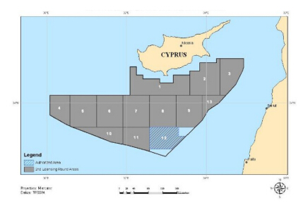
| [10] | Government of the Republic of Cyprus. Notice from the Government of the Republic of Cyprus concerning Directive 94/22/EC of the European Parliament and of the Council on the conditions for granting and using authorisations for the prospection, exploration and production of hydrocarbons. Official Journal of the European Union. C38/24, 2012. |
| [11] | Government of the Republic of Cyprus, Ministry of Commerce Industry and Tourism. "2nd Licensing round - hydrocarbon exploration". Available: http://www.mcit.gov.cy/mcit/mcit.nsf/dmlhcarbon_en/dmlhcarbon_en?OpenDocument. Cyprus, 2012. |
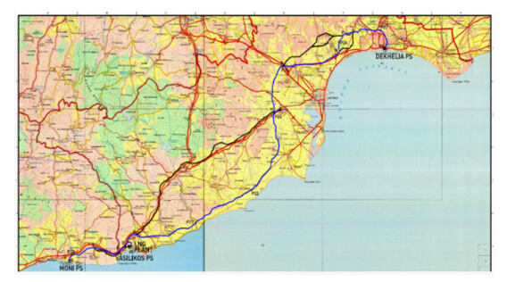
| [12] | Natural Gas Public Company (DEFA). Projects: Construction of natural gas pipeline network. Available from: http://www.defa.com.cy/en/projects.html, Cyprus, 2013. |
| [13] | European Commission, DG Energy. "Quarterly report on European Gas Markets". Volume 6, issue 1, First quarter, 2013. Available from: http://ec.europa.eu/energy/observatory/gas/doc/20130611_q1_quarterly_report_on_european_gas_markets.pdf |
| [14] | European Commission. Emissions trading: Commission adopts decision on Cyprus' national allocation plan for 2008-2012. Press Release, IP-07-1131, Brussels, July 2007. Available from: http://europa.eu/rapid/press-release_IP-07-1131_en.htm |
| [15] | European Commision. "The EU emission trading sytem EU ETS". Brussels, 2013. Available from: http://ec.europa.eu/clima/publications/docs/factsheet_ets_2013_en.pdf |
| [16] | The European Energy Exchange (EEX). "Market data on Natural Gas Spot prices and trading volumes", Frankfurt, Germany, 2013. Available from: http://www.eex.com/en/EEX |
| [17] | Statistical Service of the Cyprus Republic. "Statistical Themes: Energy, Environment". Available from: http://www.mof.gov.cy/mof/cystat/statistics.nsf/energy_environment_81main_gr/energy_environment_81main_gr?OpenForm&sub=1&sel=2 |
| [18] | Chasos, C. A., Karagiorgis G. N. and Christodoulou, C. N. (2010) Utilisation of solar/thermal power plants for production of hydrogen with applications in the transportation sector. Proceedings of the 7th Mediterranean Conference and Exhibition on Power Generation, Transmission, Distribution and Energy Conversion (MEDPOWER 2010). Agia Napa, Cyprus, 7-10 November. |
| [19] | Cyprus Organisation for Standardisation (CYS) (2008) CYS EN ISO 15403-1:2008: Natural gas — Natural gas for use as compressed fuel for vehicles — Part 1: Designation of the quality. |
| 1. | Sabrina H. Streipert, Gail S. K. Wolkowicz, Martin Bohner, Derivation and Analysis of a Discrete Predator–Prey Model, 2022, 84, 0092-8240, 10.1007/s11538-022-01016-4 | |
| 2. | A. Q. Khan, S. Khaliq, O. Tunç, A. Khaliq, M. B. Javaid, I. Ahmed, Bifurcation analysis and chaos of a discrete-time Kolmogorov model, 2021, 15, 1658-3655, 1054, 10.1080/16583655.2021.2014679 | |
| 3. | Soobia Saeed, Habibollah Haron, NZ Jhanjhi, Mehmood Naqvi, Hesham A. Alhumyani, Mehedi Masud, Improve correlation matrix of Discrete Fourier Transformation technique for finding the missing values of MRI images, 2022, 19, 1551-0018, 9039, 10.3934/mbe.2022420 | |
| 4. | Sabrina H. Streipert, Gail S. K. Wolkowicz, 2023, Chapter 22, 978-3-031-25224-2, 473, 10.1007/978-3-031-25225-9_22 | |
| 5. | Ahmad Suleman, Rizwan Ahmed, Fehaid Salem Alshammari, Nehad Ali Shah, Dynamic complexity of a slow-fast predator-prey model with herd behavior, 2023, 8, 2473-6988, 24446, 10.3934/math.20231247 | |
| 6. | Parvaiz Ahmad Naik, Muhammad Amer, Rizwan Ahmed, Sania Qureshi, Zhengxin Huang, Stability and bifurcation analysis of a discrete predator-prey system of Ricker type with refuge effect, 2024, 21, 1551-0018, 4554, 10.3934/mbe.2024201 | |
| 7. | Lijuan Niu, Qiaoling Chen, Zhidong Teng, Codimension-one bifurcation analysis and chaos control in a discrete pro- and anti-tumor macrophages model, 2024, 12, 2195-268X, 959, 10.1007/s40435-023-01241-2 | |
| 8. | Rizwan Ahmed, Abdul Qadeer Khan, Muhammad Amer, Aniqa Faizan, Imtiaz Ahmed, Complex Dynamics of a Discretized Predator–Prey System with Prey Refuge Using a Piecewise Constant Argument Method, 2024, 34, 0218-1274, 10.1142/S0218127424501207 | |
| 9. | Yashra Javaid, Shireen Jawad, Rizwan Ahmed, Ali Hasan Ali, Badr Rashwani, Dynamic complexity of a discretized predator-prey system with Allee effect and herd behaviour, 2024, 32, 2769-0911, 10.1080/27690911.2024.2420953 | |
| 10. | Parvaiz Ahmad Naik, Rizwan Ahmed, Aniqa Faizan, Theoretical and Numerical Bifurcation Analysis of a Discrete Predator–Prey System of Ricker Type with Weak Allee Effect, 2024, 23, 1575-5460, 10.1007/s12346-024-01124-7 | |
| 11. | Rizwan Ahmed, Naheed Tahir, Nehad Ali Shah, An analysis of the stability and bifurcation of a discrete-time predator–prey model with the slow–fast effect on the predator, 2024, 34, 1054-1500, 10.1063/5.0185809 | |
| 12. | Xin Wang, Jian Gao, Changgui Gu, Daiyong Wu, Xinshuang Liu, Chuansheng Shen, Composite spiral waves in discrete-time systems, 2023, 108, 2470-0045, 10.1103/PhysRevE.108.044205 | |
| 13. | Rizwan Ahmed, Muhammad Rafaqat, Imran Siddique, Mohammad Asif Arefin, A. E. Matouk, Complex Dynamics and Chaos Control of a Discrete-Time Predator-Prey Model, 2023, 2023, 1607-887X, 1, 10.1155/2023/8873611 | |
| 14. | Muhammad Asim Shahzad, Rizwan Ahmed, Dynamic complexity of a discrete predator-prey model with prey refuge and herd behavior, 2023, 11, 2309-0022, 194, 10.21015/vtm.v11i1.1512 | |
| 15. | Parvaiz Ahmad Naik, Yashra Javaid, Rizwan Ahmed, Zohreh Eskandari, Abdul Hamid Ganie, Stability and bifurcation analysis of a population dynamic model with Allee effect via piecewise constant argument method, 2024, 70, 1598-5865, 4189, 10.1007/s12190-024-02119-y |
Figures(8) / Tables(6)

Charalambos Chasos, George Karagiorgis, Chris Christodoulou. Technical and Feasibility Analysis of Gasoline and Natural Gas Fuelled Vehicles[J]. AIMS Energy, 2014, 2(1): 71-88. doi: 10.3934/energy.2014.1.71

 DownLoad:
