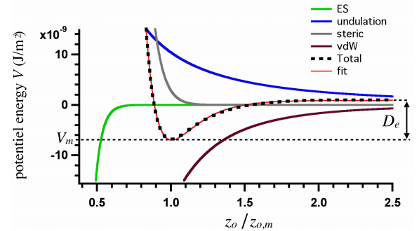
We propose a new strategy to evaluate adhesion strength at the single cell level. This approach involves variable-angle total internal reflection fluorescence microscopy to monitor in real time the topography of cell membranes, i.e. a map of the membrane/substrate separation distance. According to the Boltzmann distribution, both potential energy profile and dissociation energy related to the interactions between the cell membrane and the substrate were determined from the membrane topography. We have highlighted on glass substrates coated with poly-L-lysine and fibronectin, that the dissociation energy is a reliable parameter to quantify the adhesion strength of MDA-MB-231 motile cells.
1.
Introduction
Phytoplankton-derived carbon (internal primary production) is known to be essential for the somatic growth and reproduction of zooplankton and fish. For decades, aquatic food webs were taken as systems where carbon transfer was linear from phytoplankton to zooplankton to fish [1].
With the application of isotope labeling, substantial research shows that terrestrial organic matter (TOM) plays an important role in the lake food webs. TOM can not only affect the lake ecosystem in physical and chemical way but also can be exploited by consumer as a resource [2]. And particulate organic matter (POM) of terrestrial origin can be the key factor controlling whole-lake productivity in lakes where phytoplankton productivity is low [1,3]. Besides, in lakes, the inputs of TOM often equal to or exceed internal primary production [4].
Zooplankton composed of cladocerans, cyclopoids, and calanoids represents a critical food chain link between phytoplankton and larger fish in lakes. Lot of experimental results show that zooplankton can directly consume allochthonous POM that either entered the lake in particulate form or was formed through flocculation of allochthonous dissolved organic matter (DOM) [5]. Nevertheless, it is mentioned that Daphnia only supported by allochthonous carbon can survive and give birth to offspring [6]. For the reason that phytoplankton and zooplankton are important components of lakes, plankton mechanism considering TOM is widely studied. Lots of experiments have been done by isotope labeling [5,7,8].
Mathematical modelling is an important tool to investigate the plankton mechanism [9,10,11,12,13,14]. Nutrient-phytoplankton-zooplankton models were studied by many researchers [15,16,17]. In order to enhance the knowledge of plankton mechanism, we propose phytoplankton-zooplankton models considering TOM. We focus on the ecological function of TOM in the plankton mechanism. The results of the deterministic model can fit well with some experimental results and two hypotheses supported by experimental results in [18]. The related two hypotheses are given in the following part:
(Ⅰ) Catchment deposition hypothesis: Allochthony which is the portion of a zooplankter's body carbon content that is of terrestrial origin increases as more TOM is exported from the surrounding catchment.
(Ⅱ) Algal subtraction hypothesis: Allochthony increases with the availability of TOM, where algal production becomes limited by shading more than it benefits from the nutrients associated with TOM.
The rest of the paper is organized as follows: in the next section, by taking TOM into account, formulation of two deterministic models are discussed. In Section 3, global dynamical properties of the three-dimensional ODE model are completely established using Lyapunov function method. In Section 4, by including stochastic perturbation of the white noise type, we develop a stochastic model and show that there is a stationary distribution in the stochastic model. In Section 5, the numerical simulation is given to verify the theoretical predictions. In the biological sense, the numerical results are analyzed in detail. In the last section, the conclusion is given.
2.
Deterministic models
The research on the interaction between phytoplankton and zooplankton is important. The phytoplankton is not only the producer of the marine ecosystem but also the base of every food web. Phytoplankton is consumed by zooplankton, which is resource for consumers of higher tropical levels. By transferring organic matter and energy into higher tropical levels, zooplankton plays a critical role in lake ecosystem. Usually, the interaction between the phytoplankton and zooplankton can be described by the Prey-Predator system,
Here, P(t) and Z(t) are the population densities of phytoplankton and zooplankton, respectively. The phytoplankton grows with rate r1. The interaction term taken here is Holling type-Ⅰ with b and c as the respective rates of grazing and biomass conversion by the zooplankton for its growth such that b>c. The natural mortality of zooplankton is r2. a1 reflects the density dependence of phytoplankton. The density dependence of predator species is wildly studied because of the environment factor [14]. In lakes where phytoplankton productivity is low, zooplankton will compete each other for the resources to survive, which means that it is more realistic to consider the density dependence of zooplankton population in system (2.1). Furthermore, the zooplankton is resource for higher tropical levels. The mortality caused by higher trophic levels is generally modeled by a nonlinear term [9]. Hence, a2 reflects the density dependence of zooplankton and the mortality of zooplankton caused by higher tropic. Here, it is easy to know that system (2.1) has two equilibria: O(0,0), A(r1a1,0). Besides, when cr1−a1r2>0, there is a positive equilibrium E∗(P∗,Z∗), where P∗=r1a2+r2ba1a2+bc, Z∗=cr1−a1r2a1a2+bc, which is globally asymptotically stable. If cr1−a1r2≤0, equilibrium A(r1a1,0) is globally asymptotically stable.
Model (2.1) ignores TOM in the lake ecosystem. Since TOM has critical influence in the lake food webs, it is more realistic to incorporate it into the phytoplankton-zooplankton model. Based on the important role of TOM in lake ecosystem, we propose the terrestrial organic matter-phytoplankton-zooplankton model. The meaning of the parameters and some assumptions are proposed in following part, firstly.
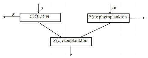
C(t) is the concentration of TOM. P(t), Z(t) are the population densities of phytoplankton and zooplankton, respectively. s is the constant input rate of TOM and δ is its sinking rate. The interaction term between the TOM and zooplankton is Holling type-Ⅰ. β0 is TOM uptake rate by zooplankton. TOM is converted for the growth of zooplankton with rate β3. The phytoplankton grows with growth rate r. K is the carrying capacity. The interaction term between the phytoplankton and zooplankton is also Holling type-Ⅰ with β1,β2 as the respective rates of grazing and biomass conversion by the zooplankton for their growth. γ is the natural mortality of zooplankton. m measures the strength of competition among zooplankton and the mortality of zooplankton caused by higher tropic. Above statements can be seen clearly in Figure 1.
Based on the above statements, the following ordinary differential equations can be derived,
In the biological context, the population densities of phytoplankton and zooplankton are nonnegative at any time t. The concentration of TOM is also nonnegative at any time t. We get the following initial conditions,
Proposition 2.1. The solution (C(t),P(t),Z(t)) of (2.2) with the initial condition (2.3) is nonnegative and bounded in R3+.
Proof. From the equations of (2.2), it is easy to get that C(t)≥C(0)e−∫t0β0Z(s)+δds≥0, P(t)=P(0)e∫t0r(1−P(s)K)−β1Z(s)ds≥0 and Z(t)=Z(0)e∫t0β2P(s)+β3C(s)−γ−mZ(s)ds≥0. Hence, the solutions are non-negative. Clearly, dCdt≤−δC+s yielding C(t)≤max{P0,sδ}:=Cmax. dPdt≤rP(1−PK) yielding P(t)≤max{K,P0}:=Pmax. Therefore, Z(t)≤β2PmaxZ+β3CmaxZ−mZ2. Hence, Z(t)≤max{Z0,β2Pmax+β3Cmaxm}. It implies the solutions (C(t),P(t),Z(t)) of (2.2) are nonnegative and bounded for all t≥0.
The nonnegativity of the solution ensures that the model has practical significance. In the following part, we can get the equilibria of (2.2). By direct calculation, it can be known that (2.2) always has two equilibria,
Proposition 2.2. If s>δγβ3, there exists unique semi-trivial equilibrium E3(C3,0,Z3) of (2.2). If K≥γβ2 and s∈(0,s1), or K<γβ2 and s∈(s0,s1), where
there exists a unique positive equilibrium E4(C4,P4,Z4).
Proof. The equilibria satisfy the following system of algebraic equations,
If P=0, Z≠0, the equilibrium is given by
where C∗ and Z∗ are constants. From the second equation of (2.5), we can get
where a3=−mβ0,b3=−(γβ0+δm),c3=β3s−γδ. If s>δγβ3, then c3>0. Thus, Δ=b23−4a3c3>0, Z31+Z32=−b3a3<0, Z31Z32=c3a3<0, which means that (2.6) exists only one positive root. It is easy to get that Z3=−b3+√b23−4a3c32a3. Then C3=γ+mZ3β3.
If P≠0,Z≠0, the equilibria of (2.4) are given by
where
If s<s1, then c4<0. Hence, H(0)=c4<0. If K≥γβ2, or K<γβ2 and s>s0, H(K)=β3s+β2Kδ−γδ>0. And limP→+∞H(P)<0. Therefore, function H(P) has two positive roots, one of which is larger than K. However, Z=rβ1(1−PK). The root which is bigger than K should be discarded. Hence, there is a unique positive equilibrium.
Here, in biologic context, E1 means that both the phytoplankton and zooplankton go extinct eventually. E2 means that the zooplankton goes extinct, while the phytoplankton will exist at the density of K eventually. E3 means that the phytoplankton goes extinct, while the zooplankton will exist at the density of Z3 eventually. E4 means that the phytoplankton and zooplankton coexist. The existence of E3 and E4 is mainly determined by s, the constant input rate of TOM.
In the next section, we will analyse the stability of those equilibria. It should be pointed out that (2.2) is totally different from the nutrient-phytoplankton-zooplankton model, for the reason that s stands for TOM, which is ingested by zooplankton.
3.
Dynamical properties of (2.2)
In this section, global dynamical properties of (2.2) are established.
Firstly, at the trivial equilibrium point E1(sδ,0,0) in (2.2), the corresponding characteristic equation is
It is apparent that equation (3.1) has one positive eigenvalue, which implies that E1(sδ,0,0) is always unstable.
Theorem 3.1. If s≥s1, then E3(C3,0,Z3) is globally asymptotically stable.
Proof. Consider the following Lyapunov function
Since the function h(z)=z−1−lnz is always nonnegative, it is easy to know that V1(t) is also nonnegative at any time t. Then the derivative of V1(t) along the solution of (2.2) is given by
If s≥s1, then β2(rβ1−Z3)≤0. It follows that dV1dt≤0. Furthermore, dV1dt=0 if and only if C(t)=C3, P(t)=0 and Z(t)=Z3. Thus, the largest invariant set on which dV1dt is zero consists of just equilibrium E3. Therefore, by LaSalle's Invariance Principle, equilibrium E3 is globally asymptotically stable.
Theorem 3.2. If K≥γβ2 and s∈(0,s1), or K<γβ2 and s∈(s0,s1), then E4(C4,P4,Z4) is globally asymptotically stable.
Proof. Consider the following Lyapunov function
Similarly, the derivative of V2(t) along the solution of (2.2) is given by
It is easy to know dV2dt≤0. dV2dt=0 if and only if C(t)=C4, P(t)=P4 and Z(t)=Z4, and hence the largest invariant set of (2.2) in the set {(C(t),P(t),Z(t))|dV2dt=0} is the singleton {E4}. Therefore, by the LaSalle's Invariance Principle, equilibrium E4 is globally asymptotically stable.
Theorem 3.3. If K<γβ2 and s∈(0,s0], then E2(sδ,K,0) is globally asymptotically stable.
Proof. Consider the following Lyapunov function
Similarly, the derivative of V3(t) along the solution of (2.2) is given by
If s≤δγβ3−β2Kδβ3, then β3C2+β2P2−γ=β3sδ+β2K−γ≤0. It is easy to know dV3dt≤0. dV3dt=0 if and only if C(t)=sδ, P(t)=K and Z(t)=0. Similarly, by the LaSalle's Invariance Principle, every solution of (2.2) tends to M, where M={(C(t),P(t),Z(t))|dV3dt=0}={E2} is the largest invariant set of (2.2). It implies that E2 is globally asymptotically stable.
Global dynamical properties of (2.2) are shown clearly in Table 1. From biological viewpoint, Theorem 3.1 implies that if the constant input of TOM is larger than s1, it will result in the extinction of phytoplankton eventually which is impossible in the system (2.1). It also means that the increasing input of the TOM will inhibit the growth of phytoplankton, which fits well with the hypotheses(Ⅱ). In addition, in the extinct process of the phytoplankton, in order to survive, the zooplankton will uptake more TOM which is easy to get. That is the Allochthony of zooplankton will increase, which fits well with the hypotheses(Ⅰ). The coexistence of TOM and zooplankton is mentioned in [6]. It also means that the producers of catchment can support both the landscape and lake ecosystem, as told in [2]. Furthermore, from Theorem 3.2, it can be known that different from the system (2.1), with the enough constant input of the TOM(s>s0), zooplankton in the deterministic setting can produce and give offsprings at small carrying capacity(K). The result fits well with the experimental result in [19]. Besides, the threshold value s1 is positively related to the birth rate of phytoplankton, which means that phytoplankton with high birth rate is less possible to become extinct. The result of Theorem 3.3 implies that zooplankton goes extinct if both the carrying capacity and constant input rate of TOM are small.
4.
Mathematical model with stochastic perturbation
In lake ecosystem, the weather, temperature and other physical factors are hard to predict. TOM, phytoplankton and zooplankton are easily affected by these factors. The deterministic model studied in the previous section does not take environmental randomness into consideration. Taking the randomness into account is more realistic. Recently, many researchers studied the stochastic biological models. Different types of stochastic perturbations are introduced into the models. Prey-predator models with fluctuations around the positive equilibrium were studied [20,21]. The stochastic perturbations which are proportional to the variables were discussed [22,23]. Fluctuations manifesting in the transmission coefficient rate were discussed [24,25].
In this section, by considering role of unpredictable environmental factors in plankton dynamics, we get following stochastic equations,
where Bi(t),i=1,2,3, are independent Brownian motions and σi, i=1,2,3 are the corresponding intensities of stochastic perturbations. Obviously, all the equilibria of (2.2) are no longer the equilibria of the stochastic model (4.1).
In this paper, let (Ω,F,{Ft}t≥0,P) be a complete probability space with filtration {Ft}t≥0 satisfying the usual conditions(i.e. it is right continuous and F0 contains all P-null sets). Let Bi(t), i=1,2,3, be a standard one-dimensional Brownian motion defined on this complete probability space. Let R3+={x∈R3:xi>0,1≤i≤3}.
Definition 4.1 ([26]). A non-negative random variable τ(ω), which is allowed to the value ∞, is called stopping time(with respect to filtration Ft), if for each t, the event {ω:τ≤t}∈Ft.
Lemma 4.2 ([26]). Let {Xt}t be right-continuous on Rn and adapted to Ft. Defineinf∅=∞. If D is an open interval on Rn, τD=inf{t≥0:Xt∉D} is a Ft stopping time.
Lemma 4.3 ([26]). Let x(t)=(x1(t),...,xn(t)) be a regular adapted process n-dimensional vector process. We can have any number n of process driven by a d-dimensional Brownian motion
where σ(t) is n×d matrix valued function, Bt is d-dimensional Brownian motion, x(t),b(t) are n-dim vector-valued functions, the integrals with respect to Brownian motion are Itˆo integrals. Then x(t) is called an Itˆo process. The only restriction is that this dependence results in:
(i) for any i=1,2...n, bi(t) is adapted and ∫T0|bi(t)|<∞ a.s..
(ii) for any i=1,2,...n, σij(t) is adapted and ∫T0σ2ij(t)<∞ a.s.
Lemma 4.4 ([27]). Let x(t) be a l-dimensional Itˆo process on t≥0 with stochastic differential
where f∈L(R+;Rl) and g∈L2(R+;Rl×m). Let V∈C2,1(Rl×R+;R). Then V(x(t),t) is till an Itˆo process with the stochastic differential given by
where
Suppose V∈C2,1(Rl×R+;R), define a operator LV from Rl×R+ to R by
Theorem 4.5. For any given initial value (C(0),P(0),Z(0))∈R3+, (4.1) has almost surely (a.s.) a unique positive solution (C(t),P(t),Z(t)) for t⩾0, and the solution remains in R3+ with probability 1.
Proof. Since the coefficients of the equation are locally Lipschitz continuous, for any given initial value (C(0),P(0),Z(0))∈R3+, it can be obtained that there is a unique local solution (C(t),P(t),Z(t)) on t∈[0,τe) where τe is the explosion time. Explosion refers to the situation when the process reaches infinite values in finite time. Solution can be considered until the time of explosion[26]. If we can check that τe=∞ a.s., then the solution is global. Let h0 be sufficient large, such that every coordinate of (C(0), P(0), Z(0)) lies within the interval [1h0,h0]. For each integer h≥h0, stopping time is defined by
where we set inf∅=∞. Clearly, τh is increasing as h→∞. Let τ∞=limh→∞τh, where τ∞≤τe a.s. If τ∞=∞ a.s., then τe=∞ and (C(t),P(t),Z(t))∈R3+ a.s. for all t≥0. If not, then it exists constants T>0 and ϵ∈(0,1) such that P{τ∞≤T}>ϵ. Hence, there is integer h1≥h0 such that
Define a function V4: R3+→R+ as
We can get the non-negativity of this function from f(u)=u+1−lnu≥0,∀u>0. Applying Itˆo formula, it follows that
Hence,
Let
Since the function f is positive, it yields ui≤2(ui+1−lnui)[23]. Therefore, β3C+β2β1(r+rK+β2)P+q3Z≤2q2V4(C,P,Z), which implies
and hence,
where q4=max{q1,2q2}. Let us define a∧b=min{a,b}. If h1≤T, then
Taking expectation of both sides, we can get that
By the Gronwall inequality,
We set Ωh={τh≤T} for h≥h1, which implies P(Ωh)≥ϵ. Note that for every ω∈Ωh, we can have that C(τh,ω) equals either h or 1h or P(τh,ω) equals either h or 1h or Z(τh,ω) equals either h or 1h, and hence,
Then it implies that
where 1Ωh is the indicator function of Ωh. Then, we let h→∞, which leads to the contradiction ∞>(V4(C(0),P(0),Z(0))+q4T)eq4T=∞. Therefore, τh=∞ a.s.
Now, we give the main result of this section in the following part.
Theorem 4.6. Assume σ21<δ, σ2, σ3>0 such that
Then there is a stationary distribution μ(⋅) for (4.1) with initial value (P0,C0,Z0)∈R3+, which has ergodic property.
Proof. Define a Lyapunov functional
Then applying Itˆo's formula to (4.1), we obtain
Since (a+b)2≤2(a2+b2), we have that
where η=β3σ21β0C4+β2σ222β1+σ232. When η<min{β3β0(δ−σ21)C4,mZ24,rβ2Kβ1P24}, we can get that the ellipsoid
lies entirely in R3+. Let U be a neighborhood of the ellipsoid with ˉU⊂El=R3+, so for x∈U∖El, LV5<−ζ(ζ is a positive constant). Therefore, we have that condition (B.2) in Lemma 2.1 of [23] is satisfied(El denotes euclidean l-space). Besides, there is M>0 such that
Thus, we have that the condition (B.1) of [23] is also satisfied. Therefore, there exists a stable stationary distribution μ(⋅) which is ergodic in (4.1).
5.
Numerical simulations
In this section, the numerical simulations of (2.2) and (4.1) are given to study the proposed models in details. Different simulated results can fit with different hypotheses mentioned in the first section. Unless otherwise stated, parameter values given in Table 2 are used for the simulations. In order to get biologically plausible results, many values are taken from parameter ranges found in the literature. And the numerical simulations of (2.2) are prepared by tool kit ode45 of Matlab.
It is easy to get s1=4.4, which is the threshold value of model (2.2). It should be noticed that since it is impossible that the absorbed energy is fully used for reproduction, the values of our parameters should satisfy β0>β3 and β1>β2. In the experimental results of [13], it points out that for zooplankton, the growth efficiency of assimilating TOM is lower than that of ingesting phytoplankton. In following analysis, hence, the values of our parameters should satisfy β1>β0.
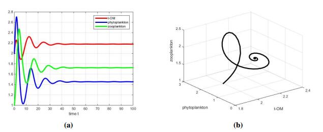
In the case where s=1<s1, Figure 2(a) shows that solutions dampen and tend to a stable steady state. The carrying capacity varies with the geographical location of the lake. Especially, the carrying capacity of poor nutrient lake is very small. If we decrease K to 1, from Theorem 3.1, we can know dynamical behavior of (2.2) is similar. However, the solution of (2.1) with the same parameter values will tend to A(r1a1,0), which means the extinction of zooplankton. Above statements can fit well with the experimental results of [28] that Daphnia magna(zooplankton) can use terrestrial-derived dissolved organic matter (t-DOM) to support growth and reproduction when alternative food sources are limiting.
The catchment areas around different lakes are different. The constant input of TOM is mainly determined by the catchment areas. It is reasonable to consider the variation of parameter value s. The values of other parameters are kept invariant.
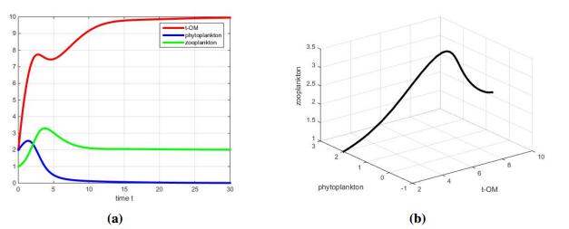
In the case where s=5>s1, we see from Figure 3(a) that the phytoplankton goes extinct eventually. In particular, because of the extinction of phytoplankton, the growth of zooplankton is determined by TOM. That is, the zooplankton shows a preference for TOM, which fits well with the hypothesis (Ⅰ).
In addition, it also means the increasing input rate of TOM will hinder the growth of phytoplankton, which fits well with the hypothesis (Ⅱ).
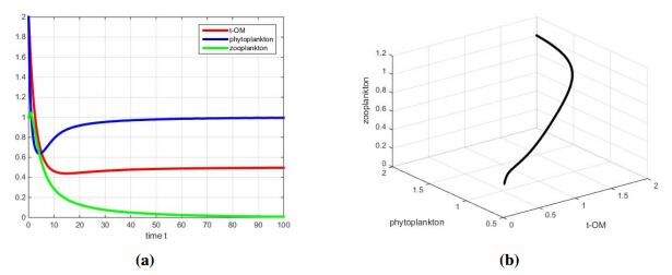
In this part, we decrease K=100 to 1 and s=1 to 0.1. The other parameter values are the same as before. The result of numerical simulation is shown in Figure 4(a). We can notice that the density of zooplankton decreases to zero, which means if both environmental capacity and constant input of TOM are small, the zooplankton goes extinct in the end.
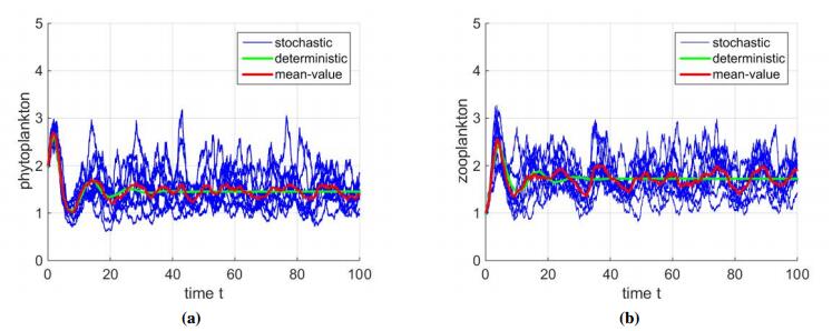
Finally, we consider the stochastic model. the values of the parameters are same as those for Figure 2. And σ1=σ2=σ3=0.1. The following discretization equations in Milsteins type[29] are used to iteratively calculate the approximate solutions of stochastic system (4.1) in Matlab programs:
where ξ1,i,ξ2,i, and ξ3,i are N(0,1)-distributed independent Gaussian random variable, σ1,σ2 and σ3 are intensities of white noise and time increment Δt>0. The simulation results are shown in Figure 5.
6.
Conclusion
In this paper, firstly, phytoplankton-zooplankton model including TOM is proposed to investigate effects of TOM upon planktonic dynamics. By constructing Lyapunov functions and using LaSalle's Invariance Principle, global stability of the equilibria which is determined by threshold values s0 and s1 is established. The analytical results of (2.2) indicate that TOM has significant effects on the lake ecosystem stability. Different constant input rates of TOM in the model can result in different results, which represents different biological meanings.
Plankton populations which reside in lake ecosystem are persistently influenced by the environmental fluctuations. In order to make more precise biological findings, we develop a stochastic model. We get that when the perturbation is small, the plankton populations reach a stationary distribution, which is ergodic. Then we simulate model (2.2) with many parameter values taken from the literature by varying the constant input rate of TOM along with the carrying capacity value. The simulations indicate that the magnitude of constant input rate of TOM and carrying capacity affect the persistence of phytoplankton populations greatly. We also simulate the stochastic model with the same parameter values. We can notice that mean value trajectory of (4.1) which is the average of ten trajectories oscillates randomly surrounding the solution of system (2.2), rather than reach the stable steady state (Figure 5). And the simulations also show that the trajectory of (4.1) is totally different from that of (2.2).
In summary, we set up exploratory models to consider the potential role of TOM that mediates interactions between trophic levels in a simple plankton food-chain. We have shown that, in principle, TOM plays an important role in influencing interactions between phytoplankton and zooplankton. The theoretical results of our deterministic model fit well with some experimental results. Further, when the perturbation is small, the stochastic model exists a stationary distribution which is ergodic. We emphasize that the qualitative behaviour of our models that we are interested in and this study are only meant as an initial exploratory attempt to consider the influence of TOM on the lake ecosystem.
Acknowledgments
This research is supported by the National Natural Sciences Foundation of China (Grant No. 11571326).
Conflict of interest
The authors declare there is no conflict of interest.


 DownLoad: