AIMS Bioengineering, 2014, 1(1): 13-24. doi: 10.3934/bioeng.2014.1.13 Research Article

Export file:

Format

RIS(for EndNote,Reference Manager,ProCite)
BibTex
Text

Content

Citation Only
Citation and Abstract

Effect of Caspase Inhibitor Ac-DEVD-CHO on Apoptosis of Vascular Smooth Muscle Cells Induced by Artesunate

Jingwen Zhang, Lu Wang, Huolin Chen, Tieying Yin, Yanqun Teng, Kang Zhang, Donghong Yu, Guixue Wang

1 Key Laboratory of Biorheological Science and Technology (Chongqing University), Ministry of Education, Chongqing Engineering Laboratory in Vascular Implants, Bioengineering College of Chongqing University, Chongqing, China, 400044.;
2 School of Bio-information Engineering, Chongqing University of Posts and Telecommunications, Chongqing, China;
3 Department of Biotechnology, Chemistry and Environmental Engineering, Aalborg University, Aalborg, Denmark

Received date: , Accepted date: , Published date:

Abstract Full Text(HTML) Figure/Table Related pages

Numerous studies have shown that the proliferation and apoptosis of vascular smooth muscle cells play a key role in restenosis. Artesunate is a triterpenoid with a peroxide structure and its antimalarial, antitumor, and antiangiogenetic activities can inhibit the proliferation and apoptosis of multifarious cells. Apoptosis is caused by the activation of a series of intracellular proteolytic enzymes, among which caspase-dependent apoptosis was the earliest to be recognized. The purpose of this article is to study the effects of caspase-3 inhibitor Ac-DEVD-CHO on proliferation and apoptosis of vascular smooth muscle cells induced by Artesunate and to explore the mechanism of Artesunate-induced apoptosis of vascular smooth muscle cells. By using the method based on methyl thiazolyl tetrazolium to observe the effects of Artesunate on the growth and proliferation of vascular smooth muscle cells; observing the change in cell shape before and after Artesunate administration by transmission electron microscopy; detecting the changes in cell cycle and apoptosis rates before and after drug administration by flow cytometry; detecting the activity of caspase-3 in the caspase apoptosis pathway by the Western Blot method, we found that Artesunate inhibits the growth and proliferation of vascular smooth muscle cells in a dose- and time-dependent manner within the concentration range of 7.5–120 μg/mL, and the inhibition rate of Artesunate can be as high as 89.49 % at a concentration of 120 μg/mL after acting for 72 hours; vascular smooth muscle cells show a typical apoptosis peak due to the effects of higher concentration of Artesunate. Compared with the control group, the higher-concentration group shows major variability, Ac-DEVD-CHO, however, can significantly decrease this induction; it has been detected by Western Blot that Artesunate can induce caspase-3 activity dramatically in vascular smooth muscle cells, but this activation may be remarkably inhibited by Ac-DEVD-CHO.

Figure/Table

Supplementary

Article Metrics

References

1. Clarke MC, Figg N, Maguire JJ, et al. (2006) Apoptosis of vascular smooth muscle cells induces features of plaque vulnerability in atherosclerosis. Nat Med 12: 1075-1080.

2. Scott S, O'Sullivan M, Hafizi S, et al. (2002) Human vascular smooth muscle cells from restenosis or in-stent stenosis sites demonstrate enhanced responses to p53: implications for brachytherapy and drug treatment for restenosis. Circ Res 90: 398-404.

3. Erl W (2005) Statin-induced vascular smooth muscle cell apoptosis: a possible role in the prevention of restenosis? Curr Drug Targets Cardiovasc Haematol Disord 5: 135-144.

4. Liu X (2006) Recent development of Artesunate. Chinese Journal of New Drugs 15:1918-1923.

5. Chen HH, Zhou HJ, Wu GD, et al. (2004) Inhibitory effects of Artesunate on angiogenesis and on expressions of vascular endothelial growth factor and VEGF receptor KDR/flk-1. Pharmacology 71: 1-9.

6. Berger TG, Dieckmann D, Efferth T, et al. (2005) Artesunate in the treatment of metastatic uveal melanoma——first experiences. Oncol Rep 14: 1599-1603.

7. Wu GD, Zhou HJ, Wu XH, et al. (2004) Apoptosis of human umbilical vein endothelial cells induced by artesunate. Vascul Pharmacol 41: 205-212.

8. He RR, Zhou HJ (2008) Progress in research on the anti-tumor effect of Artesunate. Chin J Integr Med 14: 312-316.

9. Li S, Xue F, Cheng Z, et al. (2009) Effect of Artesunate on inhibiting proliferation and inducing apoptosis of SP2/0 myeloma cells through affecting NFkappaB p65. Int J Hematol 90: 513-521.

10. Zheng JS, Wang MH, Huang M, et al. (2008) Artesunate suppresses human endometrial carcinoma RL95-2 cell proliferation by inducing cell apoptosis. Nan Fang Yi Ke Da Xue Xue Bao 28: 2221-2223.

11. Hou J, Wang D, Zhang R, et al. (2008) Experimental therapy of hepatoma with artemisinin and its derivatives: in vitro and in vivo activity, chemosensitization, and mechanisms of action. Clin Cancer Res 14: 5519-5530.

12. Sieber S, Gdynia G, Roth W, et al. (2009) Combination treatment of malignant B cells using the anti-CD20 antibody rituximab and the anti-malarial Artesunate. Int J Oncol 35: 149-158.

13. Xiao SH, Mei JY, Jiao PY (2011) Effect of mefloquine administered orally at single, multiple, or combined with artemether, Artesunate, or praziquantel in treatment of mice infected with Schistosoma japonicum. Parasitol Res 108: 399-406.

14. Keiser J, Xiao S, Smith TA, et al. (2009) Combination Chemotherapy against Clonorchis sinensis: Experiments with Artemether, Artesunate, OZ78, Praziquantel, and Tribendimidine in a Rat Model. Antimicrob Agents Chemother 53: 3770-3776.

15. Rinner B, Siegl V, Pürstner P, et al. (2004) Activity of novel plant extracts against medullary thyroid carcinoma cells. Anticancer Res 24: 495-500.

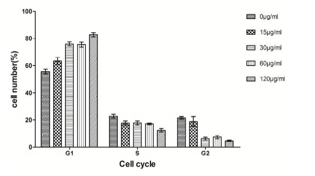
16. Zhou Z, Feng Y (2005) Artesunate reduces proliferation, interferes DNA replication and cell cycle and enhances apoptosis in vascular smooth muscle cells. J Huazhong Univ Sci Technolog Med Sci 25: 135-136.

17. Liao H (2006) Effects of Artesunate on the the proliferation and apoptosis of rat aortic vascular smooth muscle cells in vitro. Huazhong University of Science and Technology [Ph.D Dissertation].

18. Pan W, da Graca LS, Shao Y, et al. (2009) PHAPI/pp32 suppresses tumorigenesis by stimulating apoptosis. J Biol Chem 284: 6946-6954.

19. LuYY, Chen TS, Qu JL, et al. (2009) Dihydroartemisinin (DHA) induces caspase-3-dependent apoptosis in human lung adenocarcinoma ASTC-a-1 cells. J Biomed Sci 16:16.

20. Bratton SB, MacFarlane M, Cain K, et al. (2000) Protein complexes activate distinct caspase cascades in death receptor and stress-induced apoptosis. Exp Cell Res 256: 27-33.

21. Cho SG, Choi EJ (2002) Apoptotic signaling pathways: caspases and stress-activated protein kinases. J Biochem Mol Biol 35: 24-27.

22. Enari M, Sakahira H, Yokoyama H, et al. (1998) A caspase-activated DNase that degrades DNA during apoptosis, and its inhibitor ICAD. Nature 391: 43-50.

23. Korn C, Scholz SR, Gimadutdinow O, et al. (2002) Involvement of conserved histidine, lysine and tyrosine residues in the mechanism of DNA cleavage by the caspase-3 activated DNase CAD. Nucleic Acids Res 30: 1325-1332.

Copyright Info: © 2014, Guixue Wang, et al., licensee AIMS Press. This is an open access article distributed under the terms of the Creative Commons Attribution Licese (http://creativecommons.org/licenses/by/4.0)

Download full text in PDF

Export Citation

Article outline

Show full outline