Citation: Rita Shakouri, Maziar Salahi, Sohrab Kordrostami. Stochastic p-robust approach to two-stage network DEA model[J]. Quantitative Finance and Economics, 2019, 3(2): 315-346. doi: 10.3934/QFE.2019.2.315
| [1] | Salim A. Messaoudi, Mohammad M. Al-Gharabli, Adel M. Al-Mahdi, Mohammed A. Al-Osta . A coupled system of Laplacian and bi-Laplacian equations with nonlinear dampings and source terms of variable-exponents nonlinearities: Existence, uniqueness, blow-up and a large-time asymptotic behavior. AIMS Mathematics, 2023, 8(4): 7933-7966. doi: 10.3934/math.2023400 |
| [2] | Adel M. Al-Mahdi, Mohammad M. Al-Gharabli, Maher Nour, Mostafa Zahri . Stabilization of a viscoelastic wave equation with boundary damping and variable exponents: Theoretical and numerical study. AIMS Mathematics, 2022, 7(8): 15370-15401. doi: 10.3934/math.2022842 |
| [3] | Xiongmei Fan, Sen Ming, Wei Han, Zikun Liang . Lifespan estimate of solution to the semilinear wave equation with damping term and mass term. AIMS Mathematics, 2023, 8(8): 17860-17889. doi: 10.3934/math.2023910 |
| [4] | Mohammad Kafini, Jamilu Hashim Hassan, Mohammad M. Al-Gharabli . Decay result in a problem of a nonlinearly damped wave equation with variable exponent. AIMS Mathematics, 2022, 7(2): 3067-3082. doi: 10.3934/math.2022170 |
| [5] | Adel M. Al-Mahdi . The coupling system of Kirchhoff and Euler-Bernoulli plates with logarithmic source terms: Strong damping versus weak damping of variable-exponent type. AIMS Mathematics, 2023, 8(11): 27439-27459. doi: 10.3934/math.20231404 |
| [6] | Noufe H. Aljahdaly . Study tsunamis through approximate solution of damped geophysical Korteweg-de Vries equation. AIMS Mathematics, 2024, 9(5): 10926-10934. doi: 10.3934/math.2024534 |
| [7] | Mohammad Kafini, Mohammad M. Al-Gharabli, Adel M. Al-Mahdi . Existence and stability results of nonlinear swelling equations with logarithmic source terms. AIMS Mathematics, 2024, 9(5): 12825-12851. doi: 10.3934/math.2024627 |
| [8] | Zhiqiang Li . The finite time blow-up for Caputo-Hadamard fractional diffusion equation involving nonlinear memory. AIMS Mathematics, 2022, 7(7): 12913-12934. doi: 10.3934/math.2022715 |
| [9] | Muhammad Shakeel, Amna Mumtaz, Abdul Manan, Marouan Kouki, Nehad Ali Shah . Soliton solutions of the nonlinear dynamics in the Boussinesq equation with bifurcation analysis and chaos. AIMS Mathematics, 2025, 10(5): 10626-10649. doi: 10.3934/math.2025484 |
| [10] | Khaled Kefi, Nasser S. Albalawi . Three weak solutions for degenerate weighted quasilinear elliptic equations with indefinite weights and variable exponents. AIMS Mathematics, 2025, 10(2): 4492-4503. doi: 10.3934/math.2025207 |
Martínez-Jaramillo et al. (2010) argue that to maintain financial stability special attention should paid for understanding systemic risk. Even though Kanno (2015b) claims that focus on systemic risk in financial literature was earlier than the last global financial and the European debt crisis existed, and the scientific interest in systemic risk was a concern after these events. Nevertheless, until now there is no consensus on the clear concept of systemic risk or on its measurement techniques or methods (Hmissi et al., 2017).
Mendonça and Silva (2018) argue that the absence of a single clear concept of systemic risk is determined by the points of different research approaches and the choice of what the system holds and what factors influence this system. Kleinow et al. (2017a) points out that those different scholars define systemic risk based on different understandings of what a systemic risk is, and thus a measurement becomes a challenge. Moreover, the controversy causes by not having a clear systemic risk measurement and assessment methods also results in a lack of empirical research. Bisias et al. (2012) note that scholars differ in their perception of systemic risk and consequently "one cannot manage what one does not measure".
It is important to note that empirical studies can only be performed and evaluated by ex-post systemic risk. Bisias et al. (2012) emphasizes that the financial system is changing, and innovation has a major impact on it; furthermore, the author argues about the need for appropriate systemic risk measures, as research carried out at different periods in different fields and it is difficult to select one of the best or most appropriate method for assessing systemic risk. As the financial system is fluctuating and the impact of these greatly influenced by innovations, changes in the supervision and regulation of the financial system, and other challenges in the marketplace like the Big Data, the AI, IoF, blockchain, etc. Cerchiello and Giudici (2016) and Cerchiello et al. (2017) propose a novel systemic risk model, which employs both financial markets and financial tweets data using a Bayesian approach, and showed how big data can be usefully employed in modelling the financial systemic risk. Mezei and Sarlin (2016) argue that technology impact and increasing the amount of data the quantitative risk analysis and measurement make are challenging tasks. Dhar (2013) and Rönnqvist and Sarlin (2015) add, that the main challenge is how to effectively and efficiently extract meaningful information to measure the systemic risk.
Despite these facts, it is quite important to find an appropriate methods for the systemic risk assessment and measurement. This issue is particularly relevant to regulators and central banks to make the right decisions on the risk issues (Martínez-Jaramillo et al., 2010). The relevance and importance of the systemic risk analysis are also evident in the increasing research in literature, which seeks to adapt various existing systemic risk assessment methods for different countries, sectors or areas, as well as to propose new methods or approaches. The authors attempt to compare several methods and evaluate them empirically (Yun et al., 2014; Kleinow et al., 2017b; Cai et al., 2018). Nevertheless, the problem arises when new proposals, modifications of the new methods, and the empirical studies, which prove their universal acceptability to several countries or regions are lacking.
The authors (Bisias et al., 2012; Sum, 2016; Silva et al., 2017) carry out a survey of the methods to measure the systemic risk. Bisias et al. (2012) examines systematic risk assessment methods and their conceptual structures and compares them. The authors selected 31 systematic risk-measuring quantitative methods and presented open-source software implementation. The authors emphasize that the most useful methods for identifying systemic risk might be those that use regulatory authority data. The authors also argue that more than one measure needed properly assess possible threats, as systemic risk not fully understood and therefore its measurement becomes challenging. Sum (2016) conduct an analysis covering risk measurement instruments in the banking. He argues that the widespread use of the VaR model is misleading due to its cyclicality and the lack of significant accounting for events. Other alternative methods that proposed by the scholars also have positive and negative aspects. The author emphasizes that choosing the right method is very important, and it is especially relevant to improve stress-testing techniques. He also emphasizes the importance of the system against the individual risk assessment of a bank and notes the importance of establishing such models that would allow the assessment of one bank influencing and destabilizing the banking system. Silva et al. (2017) also carried out an important analysis of the literature review around systemic risk assessment. They compared 266 articles related to systemic financial risks to identify the key research and the gap that has not investigated yet. The authors emphasize that there is no clear definition of systemic risk, but risks can arise from different sources, therefore, it is important to assess and to measure systemic risk. Nevertheless, authors devote less attention comparing and analysing the methods for measuring systemic risk.
Thus, the purpose of this article is to evaluate the characteristics of the methods used to measure the systemic risk based on the literature meta-analysis and to identify their varieties and modifications.
The paper structured as follows: Section 2 provides data, research constructs, and their measurement. Section 3 divided into two sub-sections: One provides the meta-analysis of the literature on the systemic risk measurement methods, and second—presents the network maps of different systemic risk measurements based on the frequency of use of the methods, the sector, and the country, as well as the discussion of the results. Section 4 comprises a general discussion and conclusions.
The research consists of two parts: The first part dedicated to meta-analysis of the scientific literature. The second part presents the network maps that show the methods, which used to measure the systemic risk its frequency, and connections between these different methods used by various scholars in their empirical analysis.
A meta-analysis of scientific articles performed based on the Preferred Reporting Items for Systematic Reviews and Meta-Analyses (PRISMA) method (see Figure 1). This method used to select the articles published in scientific literature and to analyse the methods used to measure systemic risk. The analysis is based on data retrieved from the globally renowned database Scopus. The research covers the period of 2009–January 2018. The initial query defined by setting publication topic equal to systemic AND risk AND measure. As a result, the query returned 5888 publications. Another selection step is to exclude subject area, which is not related to the economic field like medicine, chemistry, psychology, etc. Finally, the keyword filter "systemic risk" used to select the articles. As a result, the query returned 187 publications. The duplicates publications are removed and checked the open access after those 167 publications are found available for a full download. After deeper analysis of publications, 124 articles selected for detailed research. This exclusion based on the objects or tasks of articles, which emphasized in abstracts. For example, some articles concentrate only on the theoretical literature analysis, some of them analyse narrow accounting or mathematics details, and focus on the behavioural aspects. After that we made the full text assessment. 29 articles removed from research because some of them were purely theoretical (e.g. presented only mathematical theory or derivations of formulas); publications do not have a methodology part related to the systemic risk methods or the models which are presented in those articles and do not have a clear methodology, and etc. Finally, 95 publications are analysed more deeply to determine what methods are used to measure systemic risk.
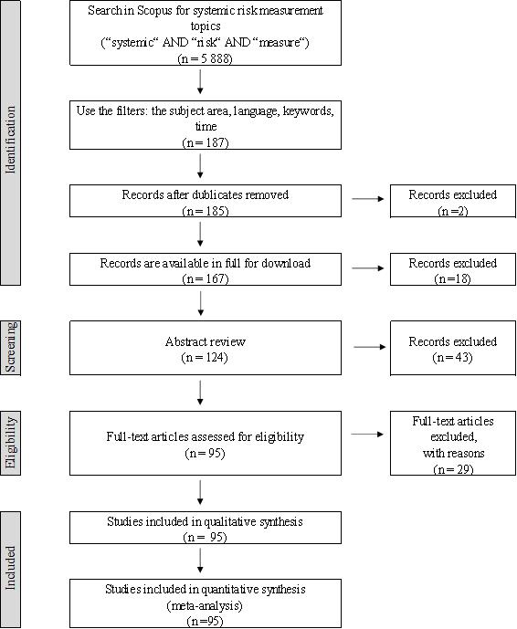 Figure 1. PRISMA method for selecting articles.
The information obtained in the first part of the study used in the second stage of the research that seeks to create the system risk measurement tools maps using a network analysis. The R Language software used to create the network maps.
Martínez-Jaramillo et al. (2010) state that systemic risk measurement and evaluation is a difficult and complex process, thus leading to a wide range of different methods and techniques to assess this risk. Scientific literature offers various methods for measuring systemic risk, creates new modifications of these methods and compares the results calculated using different ways. This abundance of methods arises the need to analyse and systematize the different systemic risk measuring methods. Thus, this part intended to examine the methods described in the scientific literature for measuring systemic risk.
As mentioned earlier 95 publications used for the study. Most of the articles used for research published in the Journal of Financial Stability, and another important part of the articles used is a research belonging to the Journal of Banking and Finance and Quantitative Finance (see Table 1).
| Source Title | Record Count | % of the total number |
| Journal of Financial Stability | 10 | 10.53% |
| Journal of Banking and Finance | 6 | 6.32% |
| Quantitative Finance | 5 | 5.26% |
| Journal of Economic Dynamics and Control | 4 | 4.21% |
| Journal of Financial Intermediation | 4 | 4.21% |
| Research in International Business and Finance | 4 | 4.21% |
| Annals of Finance | 3 | 3.16% |
| Economic Modelling | 3 | 3.16% |
| International Review of Economics and Finance | 3 | 3.16% |
| Economics Letters | 2 | 2.11% |
| European Journal of Finance | 2 | 2.11% |
| Finance a Uver—Czech Journal of Economics and Finance | 2 | 2.11% |
| Finance Research Letters | 2 | 2.11% |
| Japan and the World Economy | 2 | 2.11% |
| Journal of Empirical Finance | 2 | 2.11% |
| Journal of Financial Services Research | 2 | 2.11% |
| Journal of International Financial Markets, Institutions and Money | 2 | 2.11% |
| Journal of International Money and Finance | 2 | 2.11% |
| Pacific Basin Finance Journal | 2 | 2.11% |
| Others | 33 | 34.74% |
 DownLoad: CSV
Figure 2 shows that the interest in measuring systemic risk is increasing as the structure of the financial system changes, the quantity of innovations increases, and expanding fintech and big data. Therefore, it is important to monitor and identify the places that could lead to the systemic risk and thus undermine the stability of the financial system. According to the analysis not only the quantity of research in this area increases, but also new methods used to measure systemic risk.
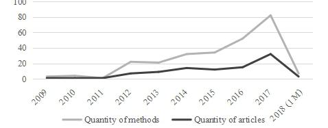 Figure 2. Publishing articles and used methods in each year, 2009–January 2018.
Figure 3 shows that the most common systemic risk measurements are the Delta conditional value-at-risk (Δ CoVaR) and the conditional value-at-risk (CoVaR) methods. Another widely used method to assess systemic risk is the Marginal Expected Shortfall (MES). It is worth mentioning that more than a fifth of the articles included in our study used the CoVaR method and about one third—the ∆ CoVaR systemic risk measurement method. The MES method has also used in more than a fifth of all analysed articles. Finally, it found that the systemic risk analysis and the application of various methods based on network methodology are particularly increased.
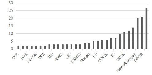 Figure 3. Frequency of methods used to measure systemic risk in analysed publications1.
1 The full names of abbreviations presented in Appendix 1.
Appendix 1 shows the results of a literature meta-analysis with presented models, methods, and other techniques, which used to assess systemic risk. We review some recent studies on systemic risk measurement in order to reveal the specific manifestations of risk measurement.
Pederzoli and Torricelli (2017) argue that systemic risk in the banking sector usually measured by two methods: CoVaR and MES. Kupiec and Güntay (2016) agree that amongst the proposed statistics, these methods are the most widely known to measure systemic risk. Pederzoli and Torricelli (2017) emphasize that these two methods derived from traditional risk-based methods: Value at Risk (VaR) and Expected Shortfall (ES). Kanno (2015a) states in his article that the value-at-risk (VaR) and expected shortfall (ES) can only applied in normal times, but not during a crisis.
First, in the case of VaR, the literature emphasizes that the most widely used the Value-at-Risk (VaR) method by the financial institutions is no longer an appropriate measure because it does not consider systemic risk profile and focuses on the risks of a single institution (Bernardi et al., 2017; Reboredo et al., 2016; Drakos et al., 2013). Kariminis and Nomikos (2017) note that needed to look for alternatives to this measure that would help to assess the risk in more systematically view and to prevent the deficiencies of VaR. Adrian and Brunnermeier (2011) suggest the Conditional Value-at-Risk (CoVaR). These authors define CoVaR how an overall VaR of the whole sector, when one institution is in distress, and Δ CoVaR defines the marginal contribution of that firm to all systemic risk.
Mendonça and Silva (2018) argue that Δ CoVaR should stand out in literature from many different systemic risk measures. The authors stress that this methodology is quite simple, and the data for analysis is publicly available. Sheu and Cheng (2012) also highlight several advantages of CoVaR and Δ CoVaR methods. They argue that this method makes it possible to see the overall risk spread across the system. Secondly, the method allows a breakdown of the marginal risk (Δ CoVaR) from all risks. In this way, it helps to draw investors' attention to the important marginal effect on risk factors, rather than all systemic risks, for example, to switch the attention from a macro prudential perspective to a micro prudential perspective. Finally, these methods can act as early warning signals for future systemic risks threats.
Other authors use the CoVar method using copula functions (Reboredo et al., 2015; Reboredo et al., 2016; Karimalis et al., 2017). Kariminis and Nomikos (2017) argue that this new proposed method for estimating CoVaR is superior since it avoids some limitations inherent in the original CoVaR model. Similarly, copula functions can overcome the stress test and sensitivity analysis, and under certain conditions, the model can train and used to investigate how a group of distress financial institutions can affect financial stability.
Girardi and Ergün (2013) expand and modify the CoVar method. López-Espinosa et al. (2015) also propose an extension of the CoVar methodology based on Adrian and Brunnermeier (2011) research. Other authors use other methods related to VaR, such as Component VaR (Liao et al., 2015), which measures the contribution of each component or factor to VaR, Incremental VaR (Liao et al., 2015), which measures changes due to changes in key risk factors, and etc.
The marginally expected shortfall (MES) method, which already has mentioned, derived from the expected shortfall (ES). Popescu and Turcu (2017) argue that MES is one of the most popular methodologies for systemic risk assessment. This is a conditional version of the ES method (Cipra et al., 2017). It formed in a similar way to CoVaR and VaR. Pederzoli and Torricelli (2017) argue that both CoVaR and MES calculations require market data that is publicly available in real time. Many methods proposed by the different scholars constructed on MES. For example, Popescu and Turcu (2017) present a novel systemic sovereign risk measure—the Expected Financing Requirements (EFR) that built on the MES. The authors seek to identify important countries and propose an adequate measuring instrument that would measure systemically not only the size of the country but also its relationship with the whole system. According to the authors, this measure provides useful information about the Eurozone countries which need more supervision over future debt repayments and whose debt is not sustainable.
Pederzoli and Torricelli (2017) conduct a study to compare the European Banking Authority (EBA) stress tests of the European banking system (published in October 2014) and market-based measures. To select MES as the market-based measure shows that the MES based on a global market index does not show a link to stress test results, while the scholars propose the Financial MES (F-MES), which based on the financial market index, and have important information and predictive power. The authors also express the view that market-based measures should be complementary to regulators, but not the main tool to test system sensitivity or perform stress tests.
Another frequently encountered measure of systemic risk: The systemic capital shortfall (SRISK). This methodology based on the MES and has become a standard to measuring systemic risk (Pederzoli et al., 2017). According to Benoit (2014), the SRISK reflects the expected capital shortfall of a certain financial institution, if the whole system affected by the crisis. In other words, the SRISK is a gap between the required capital and available capital. In this way, the banks with the greatest lack of capital become a potential source of risk. Barth and Wihlborg (2017) add that the SRISK method depends on the bank's leverage and size. Finally, although Foggitt et al. (2017) also select the SRISK method to measure systemic risk, he suggests that it be calculated using non-MES, and the long-run marginal expected shortfall (LRMES): the authors apply the Monte Carlo simulations (suggests improvements to this method).
Other systemic risk measure, based on MES, is the Component Expected Shortfall (CES). This method allows breaking down the risks of the financial system, considering the peculiarities of the institutions. Hmissi et al. (2017) state that CES, unlike the MES, can be a hybrid measuring instrument that takes both "too big to fail" and paradigm "too interconnected to fail". Meanwhile, Popescu and Turcu (2015) say that the MES and CES are complementary. When the system is struggling the MES approach shows a marginal contribution from one company to the overall downturn, while CES is the absolute contribution of this firm. The authors emphasize that these methods characterized by the fact that the data for their calculation is easily accessible, and the results of these methods are easy to interpret and understand. Banulescu and Dumitrescu (2015) argue that CES can be easily used both by regulators aiming at identifying systemically risky financial institutions and monitoring systemic risk level and by the financial institutions themselves, as they are interested in assessing their relative riskiness with a view to reducing the probability to pay a (higher) surcharge for the risk externality generated.
Kanno (2016) claims that network analysis plays a significant role to measure systemic risk. Mezei and Sarlin (2018) also argue that the recent financial crisis has led to an even greater interest in modelling and predicting the behaviour of complex financial systems. Therefore, the amount of literature on the review of the financial system as a network, rather than analyses of a separate part of the system is increasing. Kanno (2015a) concludes that to maintain the stability of the global banking system needed the systemic risk methodologies based on network approach. Authors add that such methods can used to perform stress tests for the banking system. Kanno (2015b) notes that this analysis is useful not only for scholars, but also for practitioners, for policy makers, and regulators. This analysis allows testing macro prudential policy actions. Martínez-Jaramillo et al. (2010) also emphasize that such models make it possible to exclude second-round effects according to certain simulated macroeconomic shocks.
With an increasing interest in network analysis, the number of different methods is increasing too. Souza et al. (2016) uses the DebtRank methodology and introduces a new methodology for measuring systemic risk. Silva et al. (2017) present the impact susceptibility index, which shows when market participants are vulnerable in the local market and when they can be vulnerable at a distance (remotely). The authors argue that this index proposed by them can used as a tool to monitor financial stability. The authors base their opinion on the empirical analysis of the Brazilian financial market. Mezei and Sarlin (2018) offer a new approach to measure systemic risk in networks and suggest using RiskRank.
Other authors propose new methods that allow assessing and measuring systemic risk. Kleinow et al. (2017a) offer a new method for measuring systemic risk: The Systemic Risk Index (SRI). It designed to find out the financial institution's impact on the financial sector and vice versa. Baglioni and Cherubini (2013) also offer a new index for measuring systemic default risk in the banking system: The Cuadras-Augé index. Ma and Chen (2014) construct a new financial imbalance index (FII) from the perspective of internal financial cycles. This analysis based on China's macro-financial analysis. The authors conclude that this method can be an effective indicator for measuring systemic financial risk and can provide valuable information for policy makers and market participants to make decisions.
Cambón and Estévez (2016) apply the Financial Market Stress Indicator (FMSI) in a Spanish market research. This real-time indicator quantifies the Spanish financial system's stress and quantifies the contribution of each market segment (bond market, money market, equity markets, intermediaries, and derivatives) to overall market stress. Bernardi et al. (2017) offer two new methods that summarize CoVaR and CoES: Multiple Conditional Value-at-Risk (MCoVaR) and Multiple Conditional Expected Shortfall (MCoES). According to the authors: "The proposed risk measures aim to capture extreme tail co-movements among several multivariate connected market participants experiencing contemporaneous distress instances".
Yun and Moon (2014) use MES and CoVaR methods to perform their research. The authors seek to assess how these two methods evaluate the systemic risk of an individual bank. They find that although these measures provide different ratings for systemic risk contributions, both they are a high quality and provide similar results "in explaining cross-sectional differences in systemic risk contributions across banks".
Some authors make comparisons of different methods by empirical research and draw conclusions about their reliability. Kleinow et al. (2017b) compare four market-based systemic risk measures: Marginal expected shortfall (MES), co-dependency risk (Co-Risk), delta conditional value at risk (Δ CoVaR), lower tail dependence (LTD). The authors find that differentiated methods differ in their risk assessment. The authors also add that these methodologies for measuring systemic risk offer different results when applied to small and large institutions or to different types of operating institutions (banks, affiliates or non-affiliated institutions). Moreover, they are incoherent and show completely different results. Therefore, the authors conclude that the results identifying the risks may be misleading, which means that the evaluation of risk and the measurement of it with only one method should be evaluated with caution as they may show different results.
Cai et al. (2018) use systemic capital shortfall (SRISK), distressed insurance premium (DIP) and conditional value-at-risk (CoVaR) to measure systemic risk. Authors choose these tools because they reflect different aspects of systemic risk. SRISK describes the individual banks' consequences if the whole system dropped 40 percent. DIP like SRISK shows the loss of individual banks, which depends on the expectations when aggregate banking sector falls into extreme conditions. Meanwhile, the CoVaR analysis perform vice versa. It shows the whole system of VaR, where one institution faces stress or disaster. The authors also add that the main methodological difference between these three measures is that DIP is a risk-neutral measure, while SRISK and CoVaR are statistical measures that use physical distributions.
There are many other methods presented in Appendix 1. They are also worthy of individual attention and deeper testing. As Lee et al. (2013) argue there is not one perfect methodology that would perfectly reflect the impact of disruption on the entire system. Therefore, it is very important to consider differing approaches and measurements when assessing systemic risk.
Siebenbrunner et al. (2017) raise the question of why academics and policy makers use different methods to measure systemic risk ("Why do practitioners choose a different path than academia?"). The authors argue that this is due to several reasons. First, SRISK or Δ CoVaR methods require that analysed banks to be publicly listed and have market data. Still, the problem arises that far from all banks have the necessary data, which leads to the fact that in practice practitioners simply do not apply such methods to the entire banking system. Time series also needed for a reliable model, which is also a significant obstacle. Finally, another significant reason is that academic methods and practitioners (such as capital add-ons) methods are created for different purposes.
To sum up, it is possible to say that the literature contains a very large amount of different methods for measuring systemic risk. Some authors emphasize the weaknesses or advantages of certain methods, looking for ways to improve them. Others introduce new methods or new approaches expanded and developed existing methods. Still, the appropriate method for measuring systemic risk has not yet found, which once again confirms the authors' opinion that there can be no single method or model for measuring overall systemic risk.
This part presents the network maps, that show the main interconnection of the methods used to measure systemic risk: In addition, it reveals which ones are the most widely discussed and analysed (see Figures 4–8).
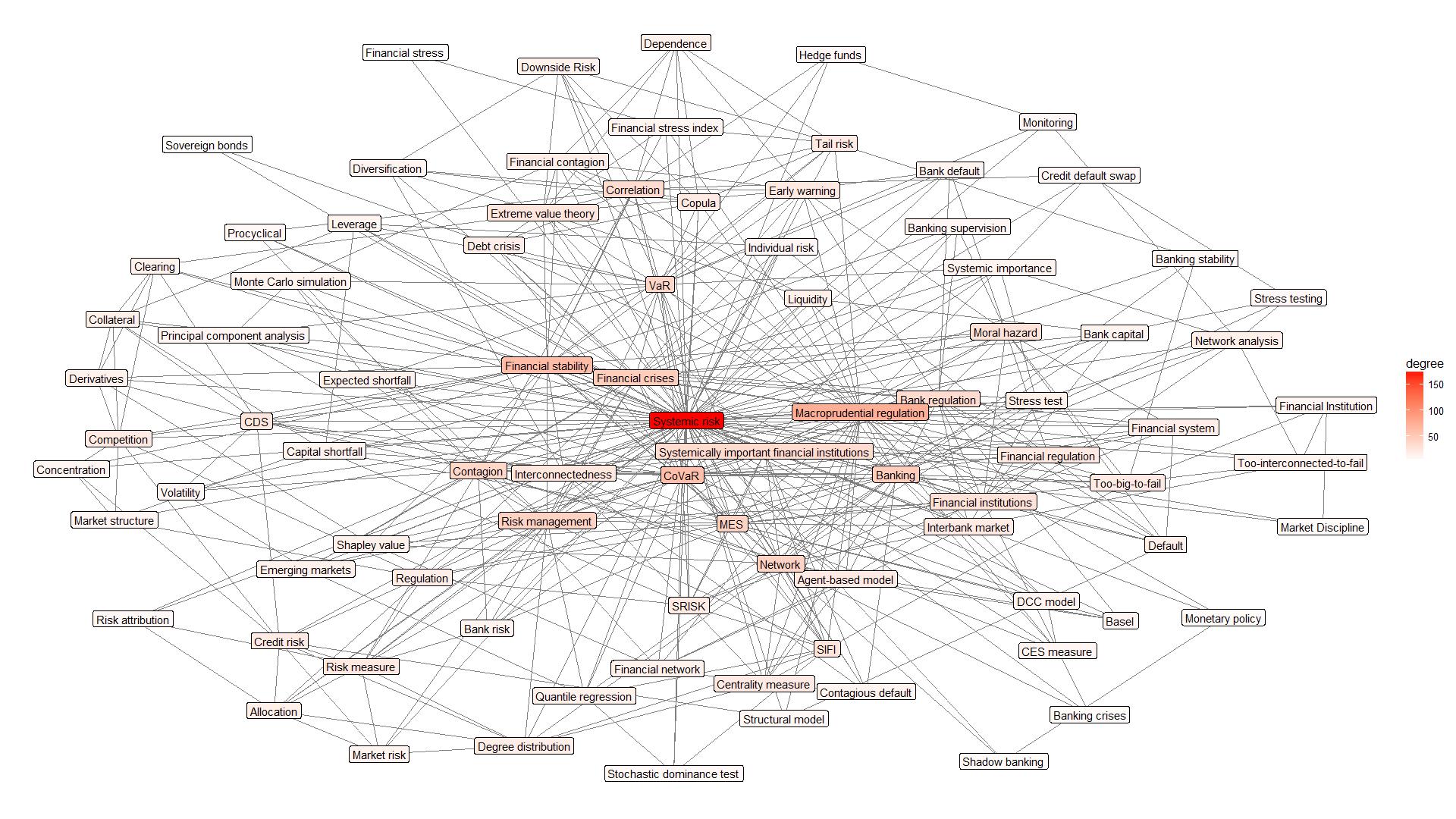 Figure 4. The network map of keywords.
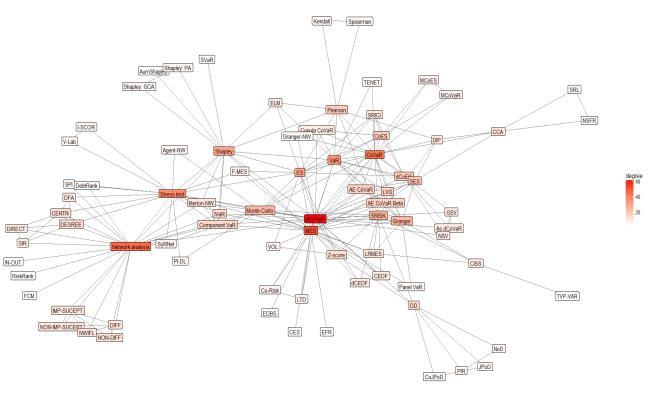 Figure 5. The network map of methods.
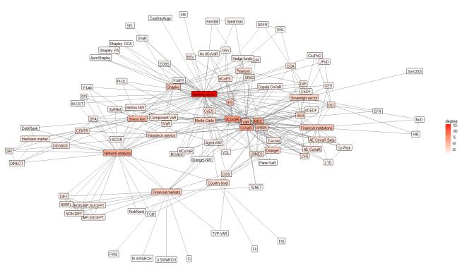 Figure 6. The network map of methods and sectors, which scholars used in their empirical research.
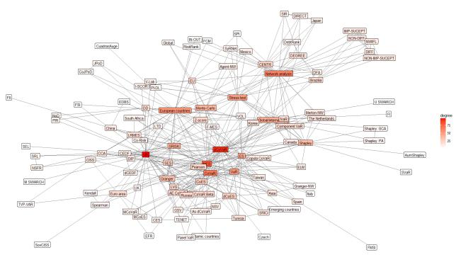 Figure 7. The network map of methods and countries/regions, which scholars used in their empirical research.
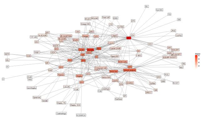 Figure 8. The network map of methods and year (based on published data of the publication).
In the first phase of the study, we analyse the keywords used by the authors themselves in the research. Figure 4 shows that most articles dealing with systemic risk are related to banking activities, financial institutions, and their size and interconnectedness, macro prudential regulation, supervision, etc. It is important to note that in scientific literature a research in shadow banking activities and its impact on financial stability is growing. Keywords map shows that the authors examining systemic risk used the keywords that define a method applied in the research. This once again confirms that it is especially important quantitatively assess systemic risk. It should emphasize that the most frequently mentioned techniques are CoVaR, MES, SRISK and Network techniques.
The network map (see Figure 5) based on those methods, which are found in literature meta-analysis. The Delta conditional value-at-risk (Δ CoVaR) is most commonly used method and compared or analysed in parallel with the MES method. The systemic risk measurement methods based on network approach also has as important part on the map (see Figure 5).
Figure 6 shows sectors and methods which are most commonly used in analysis. After the recent global crisis, attention given to the banks and their activities. Giudici and Parisi (2017) point out that the first specific methods for measuring systemic risk used to assess the banking sector. The analysis shows that scientific literature mainly focuses on the sovereign, financial markets, and institutions sector. Popescu and Turcu (2017) confirm that in the context of the crisis in the euro area countries, the focus of the research on systemic risk has shifted from banking to the sovereign sector, and it has become important to identify systemically important countries that can become critical for the whole system, union, or etc. Li and Perez-Saiz (2018) emphasize that financial market infrastructure is one of the key players in each country's financial system. Therefore, understanding the risks that arise in the network of financial market infrastructures is very important.
Less attention has paid to assessing the systemic risk on the insurance sector, as well as studies to evaluate the systemic risk of the country. However, IJtsma et al. (2017) stress that regulator is already concentrating not only on the systemic risk of an individual bank but also focused on the financial risk of the financial system in the country. Hence, the assessment of the country becomes equally important and relevant.
Finally, there are only a few empirical studies on the shadow-banking sector. As already mentioned, the analysis of scientific literature shows that the scholars apply systematic risk-taking methods and models to analyse the banking sector, but the financial system transformation focuses on the shadow banks (Aikman et al., 2017) or the activities attributable to this sector (we can see hedge funds on a map with a few research). This raises the need to expand research areas to properly and thoroughly assess systemic risk threats. Network methods mostly related to the interbank market, financial markets, and insurance sector. Meanwhile, to assess the systemic risk at the country level attempts to measure one indicator combining multiple criteria (e.g. FII, FSI), as, the banking activity based on the most widely used methods: CoVaR, VaR, MES, ΔCoVaR, etc.
It is also important to look at the countries that are being analysed as the subject of a systemic risk assessment (see Figure 7). It is noteworthy that most research aimed at examining the United States, as the recent global crisis has particularly attracted the attention of the researchers.
However, the European countries also got a considerable attention. Some scholars analyse the individual European countries, some of them only pay attention to euro-area countries or just European continent countries, and these countries groups used as different nodes. This is the reason why the European countries, compared with the USA, do not have a significant frequency in using different methods to assess systemic risk (see Figure 7).
Developing countries potentially have the greatest risks and threats. Mensah and Premaratne (2017) argue that research is mainly limited to the United States or Europe, while the Asian banking sector given too little attention. Yun and Moon (2014) also argue that research focused on these key regions, which is why the authors conduct their own research (using CoVaR and MES) on Korean Financial System. Mendonça and Silva (2018) argue that although Δ CoVaR is widely used in scientific literature, there is still a lack of research on adapting this method to developing countries. Therefore, the authors apply this method to Brazilian banking sector analysis. They argue that their analysis based on the Δ CoVaR methodology is sensitive for both bank management and changes in macroeconomic variables.
It should be noted that many innovations are started in developing countries, where is a lack of regulation and supervision, a lack of knowledge and awareness, etc. This complicates the work of both practitioners and scholars to identify and measure emerging threats and the level of these threats. The network maps analysis shows that global/international researchers are being conducted, analysing a certain aspect of the market, product or area without selecting a country for the research. Finally, Figure 8 shows that in 2017 emerge new methods, which like the new ones offered by authors and researchers themselves. Meanwhile, widely used methods such as CoVaR, MES or SRISK are the most concentrated in 2016.
Summarizing, there are many varied methods for assessing systemic risk, thus it is particularly important to choose the right methods for conducting research because different methods can show different outcomes for individual countries. There is a wide area of research to find an appropriate way of classifying systemic risk measurement methods, looking for similarities between their interconnectedness and results.
In this study, we present a comprehensive overview of the systemic risk measurement methods. In total, 95 articles selected for review and meta-analysis in the period 2009–January 2018 from the main international scientific journals accessible in Scopus database. We analyse 95 publications to determine the methods used to measure systemic risk. A meta-analysis of scientific articles performed based on the Preferred Reporting Items for Systematic Reviews and Meta-Analyses (PRISMA) method and using network approach presents the main interconnection of the methods used to measure systemic risk.
Systemic risk measurement and evaluation is a difficult and complex process and is important to monitor and identify places that could lead to systemic risk. Analysis showed that during the 2009–January 2018 not only the quantity of research in the systemic risk measurement area increases, but new methods also used to measure systemic risk. The most common systemic risk measurements are the Delta conditional value-at-risk (Δ CoVaR) and the conditional value-at-risk (CoVaR). Another widely used method to assess systemic risk is the Marginal Expected Shortfall (MES). To assess the systemic risk in the banking sector is usually used two main methods: CoVaR and MES.
CoVaR and Δ CoVaR methods make the possibility to assess the overall risk spread across the system. These methods (especially Δ CoVaR) allows a breakdown of the marginal risk from all risks, and it helps to draw investors' attention to the important marginal effect on risk factors, rather than all systemic risks. In addition, these methods can act as early warning signals for future systemic risks threats.
The network analysis also plays a crucial role to measure systemic risk, because this analysis can better model and predict the behaviour of complex financial systems. It is worth mentioning that to maintain the stability of the global banking system, the systemic risk-based methodologies needed. In addition, such type of methods can used to perform stress tests for the banking system.
It is very important to consider differing approaches and measurements when assessing systemic risk, because there is not one perfect methodology that would reflect the impact of disruption on the entire system. In addition, different methods can used to assess the systemic risk for different purposes, and from a different angle.
Finally, the network maps analysis shows the same insights as a literature meta-analysis. Most articles dealing with systemic risk, which are related to banking activities, financial institutions, and their size and interconnectedness, macro prudential regulation, supervision, etc. Keywords map shows that the authors examining systemic risk used the keywords that define a particular method applied in the research. The most frequently mentioned techniques are CoVaR, MES, SRISK and Network techniques.
The analysis in this paper has several limitations, some of which offer perspectives for future research. First, our study consists 95 papers from Scopus database and other articles (from a different database, in different languages; there were only papers in English, restricted, etc.) have not been included in this paper. Second, the new era of Big Data and other main technology challenges can significantly value added to assess the systemic risk. Future studies can link to the value and impact of these technical challenges. However, on the one hand, a large amount of data would allow for a more detailed assessment of systemic risk, but on the other, other methodologies would needed that would be more susceptible to processing large amounts of data and ability to make sense of it, i.e. potential risk. Finally, yet importantly, empirical studies should targeted by country/region, broken down into clusters, as one method may be suitable for developed countries, others for developing countries. The same logic applies to small open economies or large countries.
The authors declare no conflict of interest in this paper.
The authors gratefully thank the Deputy Editor-in Chief and the anonymous referees for their valuable comments and suggestions which have improved the paper.
| Method | 2009 | 2010 | 2011 | 2012 | 2013 | 2014 | 2015 | 2016 | 2017 | 2018 (1 M) |
| Stress test | 1 | 1 | 1 | 1 | 2 | 1 | 2 | 1 | ||
| Monte Carlo simulation | 1 | 1 | 1 | 1 | 2 | 1 | ||||
| The price of insurance against large default losses (PI–DL) | 1 | |||||||||
| Network analysis | 1 | 1 | 1 | 5 | 4 | 1 | 1 | |||
| Systemic Risk Network Model (SyRNet) | 1 | |||||||||
| A multivariate regime-switching model (the univariate SWARCH) | 1 | |||||||||
| Expected shortfall (ES) | 1 | 1 | 1 | 1 | 3 | |||||
| Pearson correlation | 1 | 1 | 1 | |||||||
| The Marginal Expected Shortfall (MES) | 1 | 2 | 1 | 1 | 5 | 10 | ||||
| Systemic contingent claims analysis (CCA) | 1 | 1 | ||||||||
| Component Value-at-Risk | 1 | 1 | ||||||||
| Incremental Value-at-Risk (IVaR) | 1 | 1 | ||||||||
| The systemic expected shortfall (SES) | 1 | 1 | ||||||||
| The Aumann-Shapley Value | 1 | |||||||||
| The Extreme Linkage Measure (ELM) | 1 | |||||||||
| The Fragility Index (FI) | 1 | |||||||||
| Value at risk (VaR) | 2 | 2 | 1 | 1 | 4 | 2 | ||||
| The conditional value-at-risk (CoVaR) | 2 | 2 | 1 | 3 | 5 | 7 | 1 | |||
| The Delta conditional value-at-risk (Δ CoVaR) | 2 | 2 | 6 | 3 | 5 | 8 | 1 | |||
| The distress insurance premium (DIP) | 2 | 1 | ||||||||
| Shapley value | 3 | 1 | 1 | 1 | ||||||
| A multivariate regime-switching model (the multivariate SWARCH) | 1 | |||||||||
| Cuadras-Augé index | 1 | |||||||||
| Network: Systemic Probability Index (SPI) | 1 | |||||||||
| Shapley value: The generalised contribution approach (GCA) | 1 | |||||||||
| Shapley value: The participation approach (PA) | 1 | |||||||||
| The non-parametric Kendall correlation | 1 | |||||||||
| Granger causality | 1 | 2 | 2 | |||||||
| The non-parametric Spearman correlation | 1 | |||||||||
| Network: The centrality measures (CENTR) | 1 | 3 | 2 | |||||||
| An agent-based network model (Agent-NW) | 1 | 1 | 1 | |||||||
| The Delta conditional Expected shortfall (Δ CoES) | 1 | 1 | 1 | |||||||
| The systemic capital shortfall (SRISK) | 1 | 2 | 7 | 1 | ||||||
| Z-score | 1 | 4 | ||||||||
| A system wide value at risk (SVaR) | 1 | |||||||||
| Financial imbalance index (FII) | 1 | |||||||||
| Gross Shapley Value (GSV) | 1 | |||||||||
| Net Shapley Value (NSV) | 1 | |||||||||
| Net Stable Funding Ratio (NSFR) | 1 | |||||||||
| The Asymmetric Delta conditional value-at-risk (As dCoVaR) | 1 | |||||||||
| The systemic risk-adjusted liquidity (SRL) model | 1 | |||||||||
| V-Lab stress test | 1 | |||||||||
| The average distance-to-default (DD)/The distance-to-default (DD) | 2 | 1 | 2 | |||||||
| Implied-Systemic Cost Of Risks (I-SCOR) index | 2 | |||||||||
| A copula conditional value-at-risk (Copula CoVaR) | 1 | 1 | 1 | |||||||
| Network: The degree distributions (DEGREE) | 1 | 1 | ||||||||
| The default analysis (DFA) | 1 | 1 | ||||||||
| A Merton style network model (Merton–NW) | 1 | |||||||||
| Network: The directed graphs (DIRECT) | 1 | |||||||||
| Network: The input–output measures (IN–OUT) | 1 | |||||||||
| Network: The modified Susceptible–Infected–Removable (SIR) model | 1 | |||||||||
| The number of joint defaults (NoD) | 1 | |||||||||
| The ratio of the price of insurance against financial distress to the aggregate asset value (PIR) | 1 | |||||||||
| The Component Expected Shortfall (CES) | 2 | 1 | ||||||||
| Composite Indicator of Systemic Stress (CISS) | 1 | 2 | ||||||||
| The conditional Expected shortfall (CoES) | 1 | 3 | ||||||||
| Adapted Exposure CoVaR (AE CoVaR) | 1 | |||||||||
| Adapted Exposure CoVaR Beta (AE CoVaR Beta) | 1 | |||||||||
| Conditional Expected Default Frequency (CEDF) | 1 | |||||||||
| Financial Market Stress Index (FMSI) | 1 | |||||||||
| Leverage (LVG) | 1 | |||||||||
| Network: DebtRank method | 1 | |||||||||
| Network: The Fuzzy Cognitive Map (FCM) | 1 | |||||||||
| Tail Event driven NETwork technique (TENET) | 1 | |||||||||
| The Delta Conditional Expected Default Frequency (Δ CEDF) | 1 | |||||||||
| Time–Varying Parameter Vector Autoregression (TVP–VAR) | 1 | |||||||||
| Co-dependency risk (Co-Risk) | 1 | |||||||||
| Expected default based score (EDBS) | 1 | |||||||||
| Financial stress index (FSI) | 1 | |||||||||
| Granger–causality network (Granger–NW) | 1 | |||||||||
| Lower tail dependence (LTD) | 1 | |||||||||
| Multiple conditional expected shortfall (MCoES) | 1 | |||||||||
| Multiple conditional Value-at-Risk (MCoVaR) | 1 | |||||||||
| Network: The non-weighted impact diffusion influence (NON–DIFF) | 1 | |||||||||
| Network: The non–weighted impact susceptibility (NON–IMP–SUCEPT) | 1 | |||||||||
| Network: The weighted impact diffusion influence (DIFF) | 1 | |||||||||
| Network: The weighted impact susceptibility (IMP–SUCEPT) | 1 | |||||||||
| Panel Value-at-Risk | 1 | |||||||||
| Systemic Risk Implication Composite Index (SRICI) | 1 | |||||||||
| The Composite Indicator of Systemic Sovereign Stress (SovCISS) | 1 | |||||||||
| The conditional joint probability of default (CoJPoD) | 1 | |||||||||
| The Expected Financing Requirements (EFR) | 1 | |||||||||
| The Financial Marginal Expected Shortfall (Financial MES) | 1 | |||||||||
| The joint probability of default (JPoD) | 1 | |||||||||
| The network impact fluidity (NWIFL) | 1 | |||||||||
| The stressed expected loss (SEL) | 1 | |||||||||
| The Systemic Risk Index (SRI) | 1 | |||||||||
| The Volatility (VOL) | 1 | |||||||||
| The long run marginal expected shortfall (LRMES) | 3 | |||||||||
| Network: RiskRank | 1 |
DownLoad: CSV| [1] |
Akther S, Fukuyama H, Weber WL (2013) Estimating two-stage network slacks-based inefficiency: An application to Bangladesh banking. Omega 41: 88–96. doi: 10.1016/j.omega.2011.02.009

|
| [2] | Alimohammadi AM, Hoseininasab H, Khademizare H, et al. (2016) A robust two-stage data envelopment analysis model for measuring efficiency: Considering Iranian electricity power production and distribution processes. Int J Eng 29: 646–653. |
| [3] |
Ang S, Chen CM (2016) Pitfalls of decomposition weights in the additive multi-stage DEA model. Omega 58: 139–153. doi: 10.1016/j.omega.2015.05.008
|
| [4] |
Avkiran NK (2009) Opening the black box of efficiency analysis: An illustration with UAE banks. Omega 37: 930–941. doi: 10.1016/j.omega.2008.08.001
|
| [5] |
Ben-Tal A, Nemirovski A (1999) Robust solutions of uncertain linear programs. Oper Res Lett 25: 1–13. doi: 10.1016/S0167-6377(99)00016-4
|
| [6] |
Ben-Tal A, Nemirovski A (2000) Robust solutions of linear programming problems contaminated with uncertain data. Math Program 88: 411–424. doi: 10.1007/PL00011380
|
| [7] |
Bertsimas D, Sim M (2003) Robust discrete optimization and network flows. Math Program 98: 49–71. doi: 10.1007/s10107-003-0396-4
|
| [8] |
Bertsimas D, Sim M (2004) The price of robustness. Oper Res 52: 35–53. doi: 10.1287/opre.1030.0065
|
| [9] |
Bertsimas D, Thiele A (2006) A robust optimization approach to inventory theory. Oper Res 54: 150–168. doi: 10.1287/opre.1050.0238
|
| [10] |
Charnes A, Cooper WW, Rhodes E (1978) Measuring the efficiency of decision making units. Eur J Oper Res 2: 429–44. doi: 10.1016/0377-2217(78)90138-8
|
| [11] |
Chen Y, Cook WD, Li N, et al. (2009) Additive efficiency decomposition in two-stage DEA. Eur J Oper Res 196: 1170–1176. doi: 10.1016/j.ejor.2008.05.011
|
| [12] | Cooper WW, Seiford LM, Tone K (2007) Data envelopment analysis: a comprehensive text with models applications references and DEA-solver software, 2nd Edition, Springer, New York. |
| [13] |
Cook WD, Liang L, Zha Y, et al. (2009) A modified super-efficiency DEA model for infeasibility. J Oper Res Soc 60: 276–281. doi: 10.1057/palgrave.jors.2602544
|
| [14] |
Cook WD, Liang L, Zhu J (2010) Measuring performance of two-stage network structures by DEA: A review and future perspective. Omega 38: 423–430. doi: 10.1016/j.omega.2009.12.001
|
| [15] | Cook WD, Zhu J (2014) Data envelopment analysis: a handbook of modeling internal structure and networks, Springer, New York, 261–284. |
| [16] |
Despotis DK, Smirlis YG (2002) Data envelopment analysis with imprecise data. Eur J Oper Res 140: 24–36. doi: 10.1016/S0377-2217(01)00200-4
|
| [17] |
Despotis DK, Sotiros D, Koronakos G (2016) A network DEA approach for series multi-stage processes. Omega 61: 35–48. doi: 10.1016/j.omega.2015.07.005
|
| [18] |
Fukuyama H, Weber WL (2010) A slacks-based inefficiency measure for a two-stage system with bad outputs. Omega 38: 398–409. doi: 10.1016/j.omega.2009.10.006
|
| [19] |
Guo C, Zhu J (2017) Non-cooperative two-stage network DEA model: Linear VS-parametric linear. Eur J Oper Res 258: 398–400. doi: 10.1016/j.ejor.2016.11.039
|
| [20] |
Gutierrez GL, Kouvelis P, Kurawarwala AA (1996) A robustness approach to incapacitated network design problems. Eur J Oper Res 94: 362–376. doi: 10.1016/0377-2217(95)00160-3
|
| [21] | Hatefi SM, Jolai F, Torabi SA, et al. (2016) Integrated forward reverse logistics network design under uncertainty and reliability consideration. Sci Iran 23: 2721–735. |
| [22] | Huang TH, Chen KC, Lin CL (2018) An extension from network DEA to Copula-based network SFA: Evidence from the U. S. commercial banks in 2009. Q Rev Econ Financ 67: 51–62. |
| [23] |
Izadikhah M, Tavana M, Caprio DD, et al. (2018) A novel two-stage DEA production model with freely distributed initial inputs and shared intermediate outputs. Expert Syst Appl 99: 213–230. doi: 10.1016/j.eswa.2017.11.005
|
| [24] |
Kao C, Hwang SN (2008) Efficiency decomposition in two stage data envelopment analysis: An application to non-life insurance companies in Taiwan. Eur J Oper Res 185: 418–429. doi: 10.1016/j.ejor.2006.11.041
|
| [25] |
Kao C, Liu S (2009) Stochastic data envelopment analysis in measuring the efficiency of Taiwan commercial banks. Eur J Oper Res 196: 312–322. doi: 10.1016/j.ejor.2008.02.023
|
| [26] |
Kao C, Liu ST (2011) Efficiencies of two-stage systems with fuzzy data. Fuzzy Set Syst 176: 20–35. doi: 10.1016/j.fss.2011.03.003
|
| [27] |
Kouvelis P, Kurawarwala AA, Gutierrez GJ (1992) Algorithms for robust single and multiple period layout planning for manufacturing systems. Eur J Oper Res 63: 287–303. doi: 10.1016/0377-2217(92)90032-5
|
| [28] |
Lewis HF, Sexton TR (2004) Network DEA: Efficiency an analysis of organizations with complex internal structure. Comput Oper Res 31: 1365–1410. doi: 10.1016/S0305-0548(03)00095-9
|
| [29] | Liang L, Yang F, Cook WD et al. (2006) DEA models for supply chain efficiency evaluation. Ann Oper Res 145: 35–49. |
| [30] |
Liang L, Wu J, Cook WD, et al. (2008) The DEA game cross-efficiency model and its Nash equilibrium. Oper Res 56: 1278–1288. doi: 10.1287/opre.1070.0487
|
| [31] |
Liang L, Cook WD, Zhu J (2008) DEA models for two-stage processes: Game approach and efficiency decomposition. Nav Res Log 55: 643–653. doi: 10.1002/nav.20308
|
| [32] | Li WH, Liang L, Cook WD (2017c) Measuring efficiency with products, by-products and parent-offspring relations: a conditional two-stage DEA model. Omega 68: 95–104. |
| [33] |
Li H, Chen C, Cook WD, et al. (2018) Two-stage network DEA: Who is the leader? Omega 74: 15–19. doi: 10.1016/j.omega.2016.12.009
|
| [34] |
Liu ST (2014) Restricting weight flexibility in fuzzy two-stage DEA. Comput Ind Eng 74: 149–160. doi: 10.1016/j.cie.2014.05.011
|
| [35] |
Lu CC (2015) Robust data envelopment analysis approaches for evaluating algorithmic performance. Comput Ind Eng 81: 78–89. doi: 10.1016/j.cie.2014.12.027
|
| [36] | Mo Y, Harrison TP (2005) A conceptual framework for robust supply chain design under demand uncertainty. Supply Chain Opt 243–263. |
| [37] |
Moreno P, Andrade GN, Meza LA, de Mello JCS (2015) Evaluation of Brazilian electricity distributors using a network DEA model with shared inputs. IEEE Latin Am Trans 13: 2209–2216. doi: 10.1109/TLA.2015.7273779
|
| [38] | Mulvey JM, Vanderbei RJ, Zenios SA (1995) Robust optimization of large-scale systems. Oper Res 43: 264–281. |
| [39] |
Paradi JC, Zhu H (2013) A survey on bank branch efficiency and performance research with data envelopment analysis. Omega 41: 61–79. doi: 10.1016/j.omega.2011.08.010
|
| [40] |
Sadjadi SJ, Omrani H (2008) Data envelopment analysis with uncertain data: An application for Iranian electricity distribution companies. Energ Policy 36: 4247–4254. doi: 10.1016/j.enpol.2008.08.004
|
| [41] |
Salahi M, Torabi N, Amiri A (2016) An optimistic robust optimization approach to common set of weights in DEA. Measurement 93: 67–73. doi: 10.1016/j.measurement.2016.06.049
|
| [42] | Salahi M, Toloo M, Hesabirad Z (2018) Robust Russell and enhanced Russell measures in DEA. J Oper Res Soc, 1–9. |
| [43] |
Seiford LM, Zhu J (1999) Profitability and marketability of the top 55 US commercial banks. Manage Sci 45: 1270–1288. doi: 10.1287/mnsc.45.9.1270
|
| [44] |
Snyder LV, Daskin MS (2006) Stochastic p-robust location problems. IIE Trans 38: 971–985. doi: 10.1080/07408170500469113
|
| [45] |
Soyster AL (1973) Convex programming with set inclusive constraints and applications to inexact linear programming. Oper Res 21: 1154–1157. doi: 10.1287/opre.21.5.1154
|
| [46] |
Thanassoulis E, Kortelainen M, Johnes G, et al. (2011) Costs and efficiency of higher education institutions in England: a DEA analysis. J Oper Res Soc 62: 1282–1297. doi: 10.1057/jors.2010.68
|
| [47] |
Tavana M, Khalili-Damghani K (2014) A new two-stage Stackelberg fuzzy data envelopment analysis model. Measurement 53: 277–296. doi: 10.1016/j.measurement.2014.03.030
|
| [48] | Wu J, Liang L (2010) Cross-efficiency evaluation approach to Olympic ranking and benchmarking: the case of Beijing 2008. Inter J App Mngt Sci 2: 76–92. |
| [49] | Wu J, Zhu Q, Chu J, et al. (2016a) Measuring energy and environmental efficiency of transportation systems in China based on a parallel DEA approach. Transp Res D Transp Environ 48: 460–472. |
| [50] | Wu J, Zhu Q, Ji X, et al. (2016b) Two-stage network processes with shared resources and resources recovered from undesirable outputs. Eur J Oper Res 251: 182–197. |
| [51] |
Wu D, Ding W, Koubaa A, et al. (2017) Robust DEA to assess the reliability of methyl methacrylate-hardened hybrid poplar wood. Ann Oper Res 248: 515–529. doi: 10.1007/s10479-016-2201-9
|
| [52] |
Yu Y, Shi Q (2014) Two-stage DEA model with additional input in the second stage and part of intermediate products as final output. Expert Syst Appl 41: 6570–6574. doi: 10.1016/j.eswa.2014.05.021
|
| [53] |
Zhou Z, Lin L, Xiao H, et al. (2017) Stochastic network DEA models for two-stage systems under the centralized control organization mechanism. Comput Ind Eng 110: 404–412. doi: 10.1016/j.cie.2017.06.005
|
Figures(3) / Tables(16)

Rita Shakouri, Maziar Salahi, Sohrab Kordrostami. Stochastic p-robust approach to two-stage network DEA model[J]. Quantitative Finance and Economics, 2019, 3(2): 315-346. doi: 10.3934/QFE.2019.2.315

| Source Title | Record Count | % of the total number |
| Journal of Financial Stability | 10 | 10.53% |
| Journal of Banking and Finance | 6 | 6.32% |
| Quantitative Finance | 5 | 5.26% |
| Journal of Economic Dynamics and Control | 4 | 4.21% |
| Journal of Financial Intermediation | 4 | 4.21% |
| Research in International Business and Finance | 4 | 4.21% |
| Annals of Finance | 3 | 3.16% |
| Economic Modelling | 3 | 3.16% |
| International Review of Economics and Finance | 3 | 3.16% |
| Economics Letters | 2 | 2.11% |
| European Journal of Finance | 2 | 2.11% |
| Finance a Uver—Czech Journal of Economics and Finance | 2 | 2.11% |
| Finance Research Letters | 2 | 2.11% |
| Japan and the World Economy | 2 | 2.11% |
| Journal of Empirical Finance | 2 | 2.11% |
| Journal of Financial Services Research | 2 | 2.11% |
| Journal of International Financial Markets, Institutions and Money | 2 | 2.11% |
| Journal of International Money and Finance | 2 | 2.11% |
| Pacific Basin Finance Journal | 2 | 2.11% |
| Others | 33 | 34.74% |
DownLoad: CSV| Method | 2009 | 2010 | 2011 | 2012 | 2013 | 2014 | 2015 | 2016 | 2017 | 2018 (1 M) |
| Stress test | 1 | 1 | 1 | 1 | 2 | 1 | 2 | 1 | ||
| Monte Carlo simulation | 1 | 1 | 1 | 1 | 2 | 1 | ||||
| The price of insurance against large default losses (PI–DL) | 1 | |||||||||
| Network analysis | 1 | 1 | 1 | 5 | 4 | 1 | 1 | |||
| Systemic Risk Network Model (SyRNet) | 1 | |||||||||
| A multivariate regime-switching model (the univariate SWARCH) | 1 | |||||||||
| Expected shortfall (ES) | 1 | 1 | 1 | 1 | 3 | |||||
| Pearson correlation | 1 | 1 | 1 | |||||||
| The Marginal Expected Shortfall (MES) | 1 | 2 | 1 | 1 | 5 | 10 | ||||
| Systemic contingent claims analysis (CCA) | 1 | 1 | ||||||||
| Component Value-at-Risk | 1 | 1 | ||||||||
| Incremental Value-at-Risk (IVaR) | 1 | 1 | ||||||||
| The systemic expected shortfall (SES) | 1 | 1 | ||||||||
| The Aumann-Shapley Value | 1 | |||||||||
| The Extreme Linkage Measure (ELM) | 1 | |||||||||
| The Fragility Index (FI) | 1 | |||||||||
| Value at risk (VaR) | 2 | 2 | 1 | 1 | 4 | 2 | ||||
| The conditional value-at-risk (CoVaR) | 2 | 2 | 1 | 3 | 5 | 7 | 1 | |||
| The Delta conditional value-at-risk (Δ CoVaR) | 2 | 2 | 6 | 3 | 5 | 8 | 1 | |||
| The distress insurance premium (DIP) | 2 | 1 | ||||||||
| Shapley value | 3 | 1 | 1 | 1 | ||||||
| A multivariate regime-switching model (the multivariate SWARCH) | 1 | |||||||||
| Cuadras-Augé index | 1 | |||||||||
| Network: Systemic Probability Index (SPI) | 1 | |||||||||
| Shapley value: The generalised contribution approach (GCA) | 1 | |||||||||
| Shapley value: The participation approach (PA) | 1 | |||||||||
| The non-parametric Kendall correlation | 1 | |||||||||
| Granger causality | 1 | 2 | 2 | |||||||
| The non-parametric Spearman correlation | 1 | |||||||||
| Network: The centrality measures (CENTR) | 1 | 3 | 2 | |||||||
| An agent-based network model (Agent-NW) | 1 | 1 | 1 | |||||||
| The Delta conditional Expected shortfall (Δ CoES) | 1 | 1 | 1 | |||||||
| The systemic capital shortfall (SRISK) | 1 | 2 | 7 | 1 | ||||||
| Z-score | 1 | 4 | ||||||||
| A system wide value at risk (SVaR) | 1 | |||||||||
| Financial imbalance index (FII) | 1 | |||||||||
| Gross Shapley Value (GSV) | 1 | |||||||||
| Net Shapley Value (NSV) | 1 | |||||||||
| Net Stable Funding Ratio (NSFR) | 1 | |||||||||
| The Asymmetric Delta conditional value-at-risk (As dCoVaR) | 1 | |||||||||
| The systemic risk-adjusted liquidity (SRL) model | 1 | |||||||||
| V-Lab stress test | 1 | |||||||||
| The average distance-to-default (DD)/The distance-to-default (DD) | 2 | 1 | 2 | |||||||
| Implied-Systemic Cost Of Risks (I-SCOR) index | 2 | |||||||||
| A copula conditional value-at-risk (Copula CoVaR) | 1 | 1 | 1 | |||||||
| Network: The degree distributions (DEGREE) | 1 | 1 | ||||||||
| The default analysis (DFA) | 1 | 1 | ||||||||
| A Merton style network model (Merton–NW) | 1 | |||||||||
| Network: The directed graphs (DIRECT) | 1 | |||||||||
| Network: The input–output measures (IN–OUT) | 1 | |||||||||
| Network: The modified Susceptible–Infected–Removable (SIR) model | 1 | |||||||||
| The number of joint defaults (NoD) | 1 | |||||||||
| The ratio of the price of insurance against financial distress to the aggregate asset value (PIR) | 1 | |||||||||
| The Component Expected Shortfall (CES) | 2 | 1 | ||||||||
| Composite Indicator of Systemic Stress (CISS) | 1 | 2 | ||||||||
| The conditional Expected shortfall (CoES) | 1 | 3 | ||||||||
| Adapted Exposure CoVaR (AE CoVaR) | 1 | |||||||||
| Adapted Exposure CoVaR Beta (AE CoVaR Beta) | 1 | |||||||||
| Conditional Expected Default Frequency (CEDF) | 1 | |||||||||
| Financial Market Stress Index (FMSI) | 1 | |||||||||
| Leverage (LVG) | 1 | |||||||||
| Network: DebtRank method | 1 | |||||||||
| Network: The Fuzzy Cognitive Map (FCM) | 1 | |||||||||
| Tail Event driven NETwork technique (TENET) | 1 | |||||||||
| The Delta Conditional Expected Default Frequency (Δ CEDF) | 1 | |||||||||
| Time–Varying Parameter Vector Autoregression (TVP–VAR) | 1 | |||||||||
| Co-dependency risk (Co-Risk) | 1 | |||||||||
| Expected default based score (EDBS) | 1 | |||||||||
| Financial stress index (FSI) | 1 | |||||||||
| Granger–causality network (Granger–NW) | 1 | |||||||||
| Lower tail dependence (LTD) | 1 | |||||||||
| Multiple conditional expected shortfall (MCoES) | 1 | |||||||||
| Multiple conditional Value-at-Risk (MCoVaR) | 1 | |||||||||
| Network: The non-weighted impact diffusion influence (NON–DIFF) | 1 | |||||||||
| Network: The non–weighted impact susceptibility (NON–IMP–SUCEPT) | 1 | |||||||||
| Network: The weighted impact diffusion influence (DIFF) | 1 | |||||||||
| Network: The weighted impact susceptibility (IMP–SUCEPT) | 1 | |||||||||
| Panel Value-at-Risk | 1 | |||||||||
| Systemic Risk Implication Composite Index (SRICI) | 1 | |||||||||
| The Composite Indicator of Systemic Sovereign Stress (SovCISS) | 1 | |||||||||
| The conditional joint probability of default (CoJPoD) | 1 | |||||||||
| The Expected Financing Requirements (EFR) | 1 | |||||||||
| The Financial Marginal Expected Shortfall (Financial MES) | 1 | |||||||||
| The joint probability of default (JPoD) | 1 | |||||||||
| The network impact fluidity (NWIFL) | 1 | |||||||||
| The stressed expected loss (SEL) | 1 | |||||||||
| The Systemic Risk Index (SRI) | 1 | |||||||||
| The Volatility (VOL) | 1 | |||||||||
| The long run marginal expected shortfall (LRMES) | 3 | |||||||||
| Network: RiskRank | 1 |
DownLoad: CSV| Source Title | Record Count | % of the total number |
| Journal of Financial Stability | 10 | 10.53% |
| Journal of Banking and Finance | 6 | 6.32% |
| Quantitative Finance | 5 | 5.26% |
| Journal of Economic Dynamics and Control | 4 | 4.21% |
| Journal of Financial Intermediation | 4 | 4.21% |
| Research in International Business and Finance | 4 | 4.21% |
| Annals of Finance | 3 | 3.16% |
| Economic Modelling | 3 | 3.16% |
| International Review of Economics and Finance | 3 | 3.16% |
| Economics Letters | 2 | 2.11% |
| European Journal of Finance | 2 | 2.11% |
| Finance a Uver—Czech Journal of Economics and Finance | 2 | 2.11% |
| Finance Research Letters | 2 | 2.11% |
| Japan and the World Economy | 2 | 2.11% |
| Journal of Empirical Finance | 2 | 2.11% |
| Journal of Financial Services Research | 2 | 2.11% |
| Journal of International Financial Markets, Institutions and Money | 2 | 2.11% |
| Journal of International Money and Finance | 2 | 2.11% |
| Pacific Basin Finance Journal | 2 | 2.11% |
| Others | 33 | 34.74% |
| Method | 2009 | 2010 | 2011 | 2012 | 2013 | 2014 | 2015 | 2016 | 2017 | 2018 (1 M) |
| Stress test | 1 | 1 | 1 | 1 | 2 | 1 | 2 | 1 | ||
| Monte Carlo simulation | 1 | 1 | 1 | 1 | 2 | 1 | ||||
| The price of insurance against large default losses (PI–DL) | 1 | |||||||||
| Network analysis | 1 | 1 | 1 | 5 | 4 | 1 | 1 | |||
| Systemic Risk Network Model (SyRNet) | 1 | |||||||||
| A multivariate regime-switching model (the univariate SWARCH) | 1 | |||||||||
| Expected shortfall (ES) | 1 | 1 | 1 | 1 | 3 | |||||
| Pearson correlation | 1 | 1 | 1 | |||||||
| The Marginal Expected Shortfall (MES) | 1 | 2 | 1 | 1 | 5 | 10 | ||||
| Systemic contingent claims analysis (CCA) | 1 | 1 | ||||||||
| Component Value-at-Risk | 1 | 1 | ||||||||
| Incremental Value-at-Risk (IVaR) | 1 | 1 | ||||||||
| The systemic expected shortfall (SES) | 1 | 1 | ||||||||
| The Aumann-Shapley Value | 1 | |||||||||
| The Extreme Linkage Measure (ELM) | 1 | |||||||||
| The Fragility Index (FI) | 1 | |||||||||
| Value at risk (VaR) | 2 | 2 | 1 | 1 | 4 | 2 | ||||
| The conditional value-at-risk (CoVaR) | 2 | 2 | 1 | 3 | 5 | 7 | 1 | |||
| The Delta conditional value-at-risk (Δ CoVaR) | 2 | 2 | 6 | 3 | 5 | 8 | 1 | |||
| The distress insurance premium (DIP) | 2 | 1 | ||||||||
| Shapley value | 3 | 1 | 1 | 1 | ||||||
| A multivariate regime-switching model (the multivariate SWARCH) | 1 | |||||||||
| Cuadras-Augé index | 1 | |||||||||
| Network: Systemic Probability Index (SPI) | 1 | |||||||||
| Shapley value: The generalised contribution approach (GCA) | 1 | |||||||||
| Shapley value: The participation approach (PA) | 1 | |||||||||
| The non-parametric Kendall correlation | 1 | |||||||||
| Granger causality | 1 | 2 | 2 | |||||||
| The non-parametric Spearman correlation | 1 | |||||||||
| Network: The centrality measures (CENTR) | 1 | 3 | 2 | |||||||
| An agent-based network model (Agent-NW) | 1 | 1 | 1 | |||||||
| The Delta conditional Expected shortfall (Δ CoES) | 1 | 1 | 1 | |||||||
| The systemic capital shortfall (SRISK) | 1 | 2 | 7 | 1 | ||||||
| Z-score | 1 | 4 | ||||||||
| A system wide value at risk (SVaR) | 1 | |||||||||
| Financial imbalance index (FII) | 1 | |||||||||
| Gross Shapley Value (GSV) | 1 | |||||||||
| Net Shapley Value (NSV) | 1 | |||||||||
| Net Stable Funding Ratio (NSFR) | 1 | |||||||||
| The Asymmetric Delta conditional value-at-risk (As dCoVaR) | 1 | |||||||||
| The systemic risk-adjusted liquidity (SRL) model | 1 | |||||||||
| V-Lab stress test | 1 | |||||||||
| The average distance-to-default (DD)/The distance-to-default (DD) | 2 | 1 | 2 | |||||||
| Implied-Systemic Cost Of Risks (I-SCOR) index | 2 | |||||||||
| A copula conditional value-at-risk (Copula CoVaR) | 1 | 1 | 1 | |||||||
| Network: The degree distributions (DEGREE) | 1 | 1 | ||||||||
| The default analysis (DFA) | 1 | 1 | ||||||||
| A Merton style network model (Merton–NW) | 1 | |||||||||
| Network: The directed graphs (DIRECT) | 1 | |||||||||
| Network: The input–output measures (IN–OUT) | 1 | |||||||||
| Network: The modified Susceptible–Infected–Removable (SIR) model | 1 | |||||||||
| The number of joint defaults (NoD) | 1 | |||||||||
| The ratio of the price of insurance against financial distress to the aggregate asset value (PIR) | 1 | |||||||||
| The Component Expected Shortfall (CES) | 2 | 1 | ||||||||
| Composite Indicator of Systemic Stress (CISS) | 1 | 2 | ||||||||
| The conditional Expected shortfall (CoES) | 1 | 3 | ||||||||
| Adapted Exposure CoVaR (AE CoVaR) | 1 | |||||||||
| Adapted Exposure CoVaR Beta (AE CoVaR Beta) | 1 | |||||||||
| Conditional Expected Default Frequency (CEDF) | 1 | |||||||||
| Financial Market Stress Index (FMSI) | 1 | |||||||||
| Leverage (LVG) | 1 | |||||||||
| Network: DebtRank method | 1 | |||||||||
| Network: The Fuzzy Cognitive Map (FCM) | 1 | |||||||||
| Tail Event driven NETwork technique (TENET) | 1 | |||||||||
| The Delta Conditional Expected Default Frequency (Δ CEDF) | 1 | |||||||||
| Time–Varying Parameter Vector Autoregression (TVP–VAR) | 1 | |||||||||
| Co-dependency risk (Co-Risk) | 1 | |||||||||
| Expected default based score (EDBS) | 1 | |||||||||
| Financial stress index (FSI) | 1 | |||||||||
| Granger–causality network (Granger–NW) | 1 | |||||||||
| Lower tail dependence (LTD) | 1 | |||||||||
| Multiple conditional expected shortfall (MCoES) | 1 | |||||||||
| Multiple conditional Value-at-Risk (MCoVaR) | 1 | |||||||||
| Network: The non-weighted impact diffusion influence (NON–DIFF) | 1 | |||||||||
| Network: The non–weighted impact susceptibility (NON–IMP–SUCEPT) | 1 | |||||||||
| Network: The weighted impact diffusion influence (DIFF) | 1 | |||||||||
| Network: The weighted impact susceptibility (IMP–SUCEPT) | 1 | |||||||||
| Panel Value-at-Risk | 1 | |||||||||
| Systemic Risk Implication Composite Index (SRICI) | 1 | |||||||||
| The Composite Indicator of Systemic Sovereign Stress (SovCISS) | 1 | |||||||||
| The conditional joint probability of default (CoJPoD) | 1 | |||||||||
| The Expected Financing Requirements (EFR) | 1 | |||||||||
| The Financial Marginal Expected Shortfall (Financial MES) | 1 | |||||||||
| The joint probability of default (JPoD) | 1 | |||||||||
| The network impact fluidity (NWIFL) | 1 | |||||||||
| The stressed expected loss (SEL) | 1 | |||||||||
| The Systemic Risk Index (SRI) | 1 | |||||||||
| The Volatility (VOL) | 1 | |||||||||
| The long run marginal expected shortfall (LRMES) | 3 | |||||||||
| Network: RiskRank | 1 |


