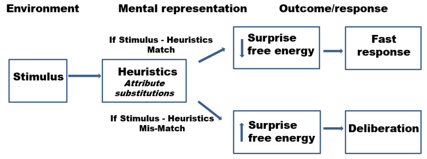
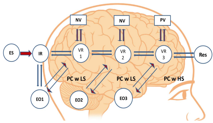
The human brain is arguably the most complex information processing system. It operates by acquiring data from the environment, recognizing patterns of events’ occurrence, anticipating their re-occurrence and in turn generating appropriate behavioral responses. Through the lenses of the free-energy principle any self-organizing system that is at equilibrium with its environment must minimize its free energy either by manipulating the environmental sensory input or by manipulating its internal states thus altering the recognition density of the outside stimuli. However, several sets of challenges interfere with the human brain's ability to learn and adapt in such a theoretically optimal fashion. These may include, and are not limited to, functional inconsistencies related to attention and memory processes, the functions of “fast” and “slow” thinking and responding, and the ability of emotional states to generate unintended behavioral outcomes that are less adaptive or inappropriate. This paper will review literature on the subject of how ideal learning viewed from the free-energy principle perspective may be affected by the above mentioned limitations and will suggest a model of information processing that may have developed as a way of overcoming these challenges. This neurobiological model stipulates that a neuronal network is formed in response to environmental input and is paralleled by at least one and possibly multiple networks that activate intrinsically and represent “virtual responses” to a situation that demands a behavioral response. This model accounts for how the brain generates a multiplicity of potential behavioral responses and may “choose” the one that seems most appropriate and also explains the uncanny ability of humans to socialize and collaborate. Implications for understanding humans’ ability to learn from others, deliberate on opposing constructs and access and utilize information outside of individual minds are also discussed.
Citation: Iliyan Ivanov, Kristin Whiteside. Dyadic Brain - A Biological Model for Deliberative Inference[J]. AIMS Neuroscience, 2017, 4(4): 169-188. doi: 10.3934/Neuroscience.2017.4.169
The human brain is arguably the most complex information processing system. It operates by acquiring data from the environment, recognizing patterns of events’ occurrence, anticipating their re-occurrence and in turn generating appropriate behavioral responses. Through the lenses of the free-energy principle any self-organizing system that is at equilibrium with its environment must minimize its free energy either by manipulating the environmental sensory input or by manipulating its internal states thus altering the recognition density of the outside stimuli. However, several sets of challenges interfere with the human brain's ability to learn and adapt in such a theoretically optimal fashion. These may include, and are not limited to, functional inconsistencies related to attention and memory processes, the functions of “fast” and “slow” thinking and responding, and the ability of emotional states to generate unintended behavioral outcomes that are less adaptive or inappropriate. This paper will review literature on the subject of how ideal learning viewed from the free-energy principle perspective may be affected by the above mentioned limitations and will suggest a model of information processing that may have developed as a way of overcoming these challenges. This neurobiological model stipulates that a neuronal network is formed in response to environmental input and is paralleled by at least one and possibly multiple networks that activate intrinsically and represent “virtual responses” to a situation that demands a behavioral response. This model accounts for how the brain generates a multiplicity of potential behavioral responses and may “choose” the one that seems most appropriate and also explains the uncanny ability of humans to socialize and collaborate. Implications for understanding humans’ ability to learn from others, deliberate on opposing constructs and access and utilize information outside of individual minds are also discussed.

| [1] |
Friston K (2010) The free-energy principle: a unified brain theory? Nat Rev Neurosci 11: 127-138. doi: 10.1038/nrn2787

|
| [2] | Jarzynski C (2012) Nonequilibrium equality for free energy differences. Phys Rev Lett 78: 2690-2693. |
| [3] | Landauer R (1996) Spatial variation of currents and fields due to localized scatterers in metallic conduction. IBM J Res Dev 1: 223-231. |
| [4] |
Sengupta B, Stemmler MB, Friston KJ (2013) Information and efficiency in the nervous system--a synthesis. PLoS Comput Biol 9: e1003157. doi: 10.1371/journal.pcbi.1003157
|
| [5] |
Simons DJ, Chabris CF (2011) What people believe about how memory works: a representative survey of the U.S. population. PLoS One 6: e22757. doi: 10.1371/journal.pone.0022757
|
| [6] |
Friston K, FitzGerald T, Rigoli F, et al. (2016) Active inference and learning. Neurosci Biobehav Rev 68: 862-879. doi: 10.1016/j.neubiorev.2016.06.022
|
| [7] |
Friston K, Rigoli F, Ognibele D, et al. (2015) Active inference and epistemic value. Cogn Neurosci 6: 187-214. doi: 10.1080/17588928.2015.1020053
|
| [8] |
Ognibene D, Chinellato E, Sarabia M, et al. (2013) Contextual action recognition and target localization with an active allocation of attention on a humanoid robot. Bioinspir Biomim 8: 035002. doi: 10.1088/1748-3182/8/3/035002
|
| [9] | Kahneman D (2011) Thinking, fast and slow. New York, NY. |
| [10] |
Clark A, Chalmers DJ (1998) The extended mind. Analysis 58: 7-19. doi: 10.1093/analys/58.1.7
|
| [11] | Kahneman D, Frederick S (2002) Representativeness revisited: Attribute substitution in intuitive judgment. In Gilovich T, Griffin D, Kahneman, D (Eds), Heuristics and biases: The psychology of intuitive judgment, New York, NY: 49-81. |
| [12] |
Kahneman D (2003) Maps of bounded rationality: Psychology for behavioral economics. American Economic Review 93: 1449-1475. doi: 10.1257/000282803322655392
|
| [13] |
Simon HA (1955) A behavioral model of rational choice. Quarterly Journal of Economics 69: 99-118. doi: 10.2307/1884852
|
| [14] | Lerner RG, Trigg GL (1991) Encyclopedia of Physics (2nd Edition). New York, NY: VCH Publishers. |
| [15] | Parker CB (1994) McGraw-Hill Encyclopedia of Physics (2nd Edition). New York, NY: McGraw-Hill. |
| [16] | Penrose R (2007) The Road to Reality: A Complete Guide to the Laws of the Universe. New York, NY: Vintage Books. |
| [17] |
Panksepp J (2005) Affective consciousness: core emotional feelings in animals and humans. Conscious Cogn 14: 30-80. doi: 10.1016/j.concog.2004.10.004
|
| [18] | Boltzmann L (1877) U ̈ er die beziehung zwischen dem zweiten haupt- satz der mechanischen wa ̈rmetheorie und der wahrscheinlichkeitsrech- nung respektive den sa ̈tzen u ̈ber das wa ̈rmegleichgewicht. [On the relationship between the second law of the mechanical theory of heat and the probability calculus]. Wiener Berichte 76: 373-435. |
| [19] | Wiener N (1961) Cybernetics-or control and communication in the animal and the machine. New York, NY. |
| [20] |
Hirsh JB, Mar RA, Peterson JB (2012) Psychological entropy: A framework for understanding uncertainty-related anxiety. Psychol Rev 119: 304-320. doi: 10.1037/a0026767
|
| [21] |
Keysers C (2009) Mirror neurons. Curr Biol 19: 971-973. doi: 10.1016/j.cub.2009.08.026
|
| [22] | Molenberghs P, Cunnington R, Mattingley JB (2009) Is the mirror neuron system involved in imitation? A short review and meta-analysis. Neurosci Biobehav Rev 33: 975-980. |
| [23] |
Rizzolatti G, Craighero L (2004) The mirror-neuron system. Ann Rev Neurosci 27: 169-192. doi: 10.1146/annurev.neuro.27.070203.144230
|
| [24] |
Filimon F, Rieth CA, Sereno MI, et al. (2015) Observed, executed, and imagined action representations can be decoded from ventral and dorsal areas. Cereb Cortex 25: 3144-3158. doi: 10.1093/cercor/bhu110
|
| [25] |
Trapp K, Spengler S, Wüstenberg T, et al. (2014) Imagining triadic interactions simultaneously activates mirror and mentalizing systems. Neuroimage 98: 314-323. doi: 10.1016/j.neuroimage.2014.05.003
|
| [26] | Felleman DJ, Van Essen DC (1991) Distributed hierarchical processing in the primate cerebral cortex. Cereb Cortex 1: 1-47. |
| [27] |
von Stein A, Sarnthein J (2000) Different frequencies for different scales of cortical integration: from local gamma to long range alpha/theta synchronization. Int J Psychophysiol 38: 301-313. doi: 10.1016/S0167-8760(00)00172-0
|
| [28] |
Réka Albert AB (2002) Statistical mechanics of complex networks. Rev Mod Phys 74: 47-97. doi: 10.1103/RevModPhys.74.47
|
| [29] | Amit DJ (1995) The Hebbian paradigm reintegrated: local reverberations as internal representations. Behav Brain Sci 18: 631. |
| [30] |
Goldman-Rakic PS (1995) Cellular basis of working memory. Neuron 14: 477-485. doi: 10.1016/0896-6273(95)90304-6
|
| [31] |
Wang XJ (2001) Synaptic reverberation underlying mnemonic persistent activity. Trends Neurosci 24: 455-463. doi: 10.1016/S0166-2236(00)01868-3
|
| [32] |
Trantham-Davidson H, Neely LC, Lavin A, et al. (2004) Mechanisms underlying differential D1 versus D2 dopamine receptor regulation of inhibition in prefrontal cortex. J Neurosci 24: 10652-10659. doi: 10.1523/JNEUROSCI.3179-04.2004
|
| [33] |
Stephens GJ, Silbert LJ, Hasson U (2010) Speaker–listener neural coupling underlies successful communication. Proc Natl Acad Sci U S A 107: 14425-14430. doi: 10.1073/pnas.1008662107
|
| [34] |
Hasson U, Ghazanfa AA, Galantucci B, et al. (2012) Brain-to-brain coupling: a mechanism for creating and sharing a social world. Trends Cogn Sci 16: 114-121. doi: 10.1016/j.tics.2011.12.007
|
| [35] |
Benoit RG, Gilbert SJ, Frith CD, et al. (2012) Rostral prefrontal cortex and the focus of attention in prospective memory. Cereb Cortex 22: 1876-1886. doi: 10.1093/cercor/bhr264
|
| [36] |
Nader K, Schafe GE, Le Doux JE (2000) Fear memories require protein synthesis in the amygdala for reconsolidation after retrieval. Nature 406: 722-726. doi: 10.1038/35021052
|
| [37] |
Przybyslawski J, Sara SJ (1997) Reconsolidation of memory after its reactivation. Behav Brain Res 84: 241-246. doi: 10.1016/S0166-4328(96)00153-2
|
| [38] |
Sara SJ (2000) Retrieval and reconsolidation: toward a neurobiology of remembering. Learn Mem 7: 73-84. doi: 10.1101/lm.7.2.73
|
| [39] | Colarusso CA, Nemiroff RA (1981) Adult Development: A New Dimension in Psychodynamic Theory and Practice. New York, NY: Plenum. |
| [40] |
Pennisi E (2010) Conquering by copying. Science 328: 165-167. doi: 10.1126/science.328.5975.165
|
Figures(2)

Iliyan Ivanov, Kristin Whiteside. Dyadic Brain - A Biological Model for Deliberative Inference[J]. AIMS Neuroscience, 2017, 4(4): 169-188. doi: 10.3934/Neuroscience.2017.4.169


 DownLoad: