Research article Recurring Topics

Relevance of Brain-derived Neurotrophic Factor Levels in Schizophrenia: A Systematic Review and Meta-Analysis

  • Received: 23 April 2015 Accepted: 14 November 2015 Published: 18 November 2015
  • Background: Brain Derived Neurotrophic Factor (BDNF) is one of the neuromodulators crucial for the survival, development and function of neurones in the brain and nervous system. Several authors linked its changes in production and concentration to Schizophrenia syndromes. Aim: This systematic review examined the available evidence to clarify the association between plasma BDNF levels and Schizophrenia. Method: Initial searches revealed 266 records. After screening of abstracts, 20 studies were selected. Following a preliminary review, 14 studies were included in this systematic review and meta-analysis. Results: Of the 14 studies (910 patients, 717 controls) 8 reported decreased BDNF levels in patients with schizophrenia as compared to controls; 3 studies (274/128) found increased BDNF levels; while 3 (62/62) reported no group differences. Meta-analysis of all pooled studies confirmed reduced BDNF levels in schizophrenia versus controls (medium effect size); however, the group difference was not significant when studies using unmedicated cases were considered. Conclusion: The cumulative evidence indicates reduced BDNF levels existing in schizophrenia. However, findings are less clear in unmedicated cases, suggesting that reduced BDNF levels in schizophrenia may be associated with symptom chronicity and/or chronic effects of antipsychotic medication.

    Citation: Ian M Rowbotham, Franco F Orsucci, Mohamed F Mansour, Samuel R Chamberlain, Haroon Y Raja. Relevance of Brain-derived Neurotrophic Factor Levels in Schizophrenia: A Systematic Review and Meta-Analysis[J]. AIMS Neuroscience, 2015, 2(4): 280-293. doi: 10.3934/Neuroscience.2015.4.280

    Related Papers:

    [1] Shengyu Huang, Hengguo Yu, Chuanjun Dai, Zengling Ma, Qi Wang, Min Zhao . Dynamics of a harvested cyanobacteria-fish model with modified Holling type Ⅳ functional response. Mathematical Biosciences and Engineering, 2023, 20(7): 12599-12624. doi: 10.3934/mbe.2023561
    [2] Ali Moussaoui, Pierre Auger, Christophe Lett . Optimal number of sites in multi-site fisheries with fish stock dependent migrations. Mathematical Biosciences and Engineering, 2011, 8(3): 769-783. doi: 10.3934/mbe.2011.8.769
    [3] Shengyu Huang, Hengguo Yu, Chuanjun Dai, Zengling Ma, Qi Wang, Min Zhao . Dynamic analysis of a modified algae and fish model with aggregation and Allee effect. Mathematical Biosciences and Engineering, 2022, 19(4): 3673-3700. doi: 10.3934/mbe.2022169
    [4] Pierre Auger, Tri Nguyen-Huu, Doanh Nguyen-Ngoc . On the impossibility of increasing the MSY in a multisite Schaefer fishing model. Mathematical Biosciences and Engineering, 2025, 22(2): 415-430. doi: 10.3934/mbe.2025016
    [5] Xiang Nan, Kayo kanato . Role of information security-based tourism management system in the intelligent recommendation of tourism resources. Mathematical Biosciences and Engineering, 2021, 18(6): 7955-7964. doi: 10.3934/mbe.2021394
    [6] Yuanpei Xia, Weisong Zhou, Zhichun Yang . Global analysis and optimal harvesting for a hybrid stochastic phytoplankton-zooplankton-fish model with distributed delays. Mathematical Biosciences and Engineering, 2020, 17(5): 6149-6180. doi: 10.3934/mbe.2020326
    [7] Sheree L. Arpin, J. M. Cushing . Modeling frequency-dependent selection with an application to cichlid fish. Mathematical Biosciences and Engineering, 2008, 5(4): 889-903. doi: 10.3934/mbe.2008.5.889
    [8] Carlos Camilo-Garay, R. Israel Ortega-Gutiérrez, Hugo Cruz-Suárez . Optimal strategies for a fishery model applied to utility functions. Mathematical Biosciences and Engineering, 2021, 18(1): 518-529. doi: 10.3934/mbe.2021028
    [9] Huidong Cheng, Hui Xu, Jingli Fu . Dynamic analysis of a phytoplankton-fish model with the impulsive feedback control depending on the fish density and its changing rate. Mathematical Biosciences and Engineering, 2023, 20(5): 8103-8123. doi: 10.3934/mbe.2023352
    [10] Yuan Tian, Yan Gao, Kaibiao Sun . A fishery predator-prey model with anti-predator behavior and complex dynamics induced by weighted fishing strategies. Mathematical Biosciences and Engineering, 2023, 20(2): 1558-1579. doi: 10.3934/mbe.2023071
  • Background: Brain Derived Neurotrophic Factor (BDNF) is one of the neuromodulators crucial for the survival, development and function of neurones in the brain and nervous system. Several authors linked its changes in production and concentration to Schizophrenia syndromes. Aim: This systematic review examined the available evidence to clarify the association between plasma BDNF levels and Schizophrenia. Method: Initial searches revealed 266 records. After screening of abstracts, 20 studies were selected. Following a preliminary review, 14 studies were included in this systematic review and meta-analysis. Results: Of the 14 studies (910 patients, 717 controls) 8 reported decreased BDNF levels in patients with schizophrenia as compared to controls; 3 studies (274/128) found increased BDNF levels; while 3 (62/62) reported no group differences. Meta-analysis of all pooled studies confirmed reduced BDNF levels in schizophrenia versus controls (medium effect size); however, the group difference was not significant when studies using unmedicated cases were considered. Conclusion: The cumulative evidence indicates reduced BDNF levels existing in schizophrenia. However, findings are less clear in unmedicated cases, suggesting that reduced BDNF levels in schizophrenia may be associated with symptom chronicity and/or chronic effects of antipsychotic medication.


    The sustainable management of marine ecosystems is paramount for ensuring the well-being of coastal communities and the preservation of biodiversity [1]. It is crucial to examine how the global community can address the gap in marine economy and marine tourism development by leveraging their expertise, innovation, capabilities, and financial resources to prevent underdeveloped nations from falling behind in the realm of sustainable marine economy [2]. Coastal and marine tourism constitutes a crucial aspect of a sustainable blue economy, generating employment for millions of individuals [3]. Tourism is considered a sustainable and environmentally friendly option, forming a mutually beneficial relationship with the ecosystem over time [4]. Furthermore, it is characterized as a "smokeless industry", leveraging social, historical, physical, and cultural resources. Projections suggest a worldwide expansion of $ 3.5\% $ in the ocean economy and marine tourism sector [5]. By 2030, marine and coastal tourism are anticipated to emerge as the primary value-added segment of the marine economy, comprising $ 26\% $ of total production [6]. However, increasing evidence suggests that high human visitation rates in natural areas can lead to significant environmental impacts, mainly due to the scale and concentration of tourism activities [7,8]. For instance, globally, terrestrial protected areas receive billions of visits annually, generating substantial revenue and posing threats to native wildlife due to infrastructure development and access facilitation for large crowds [9,10]. One notable example is the Great Smoky Mountains National Park, which attracts over ten million visitors per year in the USA [11]. Several researchers [12,13] have raised concerns about this matter, with Hall and McArthur [14] characterizing it as a paradoxical situation.

    Fishing also serves as a significant and sustainable means of livelihood, as highlighted in a recent report by the Food and Agriculture Organization (FAO) [15]. The report indicates that nearly 38.98 million individuals are engaged in fishing, contributing to approximately 7% of the global protein supply sourced from seafood. However, despite its importance, coastal communities reliant on fisheries face many challenges stemming from social, economic, political, and environmental factors [16,17]. The exacerbation of these issues by anthropogenic climate change and the overexploitation of marine resources intensifies the pressure on these communities and their fishing sectors [18,19,20]. Acknowledging the inherent intricacy and unpredictability, fisheries management strategies should adopt intricate marine socio-ecological-economic systems (SEESs) [21,22]. However, traditional linear decision-making processes often fail to address the complexity of SEESs, leading to recurring management problems [23]. The Ecosystem approach to fisheries management (EAFM), widely adopted in governing these SEESs, seeks to holistically manage capture fisheries to ensure healthy marine ecosystems and sustainable livelihoods derived from fishing activities [24,25]. Such an approach actively promotes sustainable thinking and stakeholder participation to address these challenges [26,27]. Effective implementation of the EAFM requires balancing multiple objectives and considering priorities and trade-offs in a multi-stakeholder context [28,29], emphasizing the integration of various criteria to support decision-making processes.

    Wetlands, termed the "kidneys of the earth", are crucial ecological components, now recognized for their role in environmental diversity and supported by the rise of fishing and ecotourism [30]. However, their development has suffered from exploitation, resulting in environmental harm [31,32]. Preserving ecosystem balance is essential for sustainable development to prevent reduced species diversity, resource depletion, and environmental degradation [33,34]. Fortunately, growing awareness among the public and government has spurred concerted actions towards wetland conservation and sustainable fishing and ecotourism [35]. Enforcing regulatory policies concerning fishing activities and ecotourism is crucial for striking a delicate equilibrium between economic progress and ecological sustainability [36]. Fishing tax and tourist entrance fee policies are vital for regulating fishing activities and promoting sustainable tourism practices in wetland ecosystems [37,38]. These policies influence the behavior of fishers, tourism operators, and consumers, shaping the dynamics of resource utilization and revenue generation [39]. By strategically adjusting fishing taxes and tourist entrance fees, governing bodies can incentivize sustainable fishing practices, reduce overfishing, and mitigate the negative impacts of tourism on marine habitats [40]. The implementation of such regulating policies supports sustainable development goals (SDGs) 8 and 14, promoting decent work, economic growth, and sustainable marine ecosystems, thereby aiding poverty reduction and economic development in coastal communities, particularly for fishers and tourism stakeholders [41]. Furthermore, these policies foster a sustainable blue economy and contribute to other SDGs such as SDG 1, 2, 13, and 15 by enhancing food security, poverty alleviation, climate resilience, and biodiversity conservation in coastal regions, promoting holistic and sustainable development [42].

    Numerous studies have been undertaken in this direction to explore research and its implications. Cohen-Shacham et al. [43] performed a stakeholder analysis at the Galilee Sea Hula wetland, revealing that insufficient coordination among stakeholders could result in competition for cultural services, particularly tourism, jeopardizing habitat services like biodiversity conservation. Boncoeur et al. [44] examined the bioeconomic effects of both ecotourism and fishing and found that the introduction of a marine reserve alongside a fishing zone brings about more intricate economic outcomes than expected by studies concentrating solely on one stock and/or commercial fisheries. Kar and Ghosh [45] investigated the financial implications and sustainability of reserve areas involving multiple species and activities, suggesting that the combined revenue from ecotourism and fisheries could surpass that from fisheries alone. Gallagher and Hammerschlag [46] examined a South African shark tourism operation, analyzing 12 years of demographic and economic data, uncovering rising trends in customer numbers and trip costs. They highlighted the economic potential of shark-based tourism, benefiting national economies. Lee and Iwasa [47] optimized tourist entrance fees in a shared fishing and ecotourism area, demonstrating that resource availability significantly impacts benefit distribution among stakeholders. In contrast, in a comparable fishing area, Sarkar et al. [48] primarily concentrated on optimizing fishing taxes while keeping tourist entrance fees constant. Many other studies have been conducted in this direction, focusing solely on either fishing management or ecotourism governance [49,50,51,52,53]. Despite recent progress, the impacts of ecotourism and fishing on ecosystems with multiple species and activities remain largely unexplored. Researchers mainly focus on decentralized decision-making schemes (DDMS), characterized by challenges such as lack of coordination, suboptimal resource allocation, and inefficiencies due to independent optimization of control parameters [54]. This underscores the importance of a centralized decision-making scheme (CDMS) enabling coordinated governance strategies for optimizing resource allocation and promoting ecosystem sustainability [55]. Therefore, we seek to investigate a two-parameter dynamic optimization approach within a CDMS to comprehensively understand system dynamics and societal benefits.

    We build upon the classical predator-prey framework, extending it to incorporate harvesting dynamics and fishery-based tourism. Predator-prey models have been extensively studied in ecological modeling, with recent advancements focusing on nonlocal interactions, functional responses, and behavioral effects [56,57]. For instance, bifurcation phenomena in modified Leslie-Gower systems with nonlocal competition and Beddington-DeAngelis functional response have been explored in Ma and Yang [58], while the influence of fear effects in such models has been analyzed in Zhu and Yang [59]. Chatterjee et al. [60] examined the dynamic behavior of a predator-prey model in the presence of migratory prey and predator preference. Ghorai et al. [61] further examined the effect of preferential selection of predators and the spatiotemporal patterns formation in the predator-prey model. A predator-prey model with prey refuge was studied under a stochastic and deterministic environment in [62]. Here, we investigate the socio-ecological-economic implications of regulatory policies to preserve fisheries and ecotourism activities within a predator-prey ecological framework. Specifically, we explore implementing a taxation fee system for managing a fishing zone alongside a no-take zone within a region governed by a tourist entry fee system inhabited by interdependent prey (fish) and predator (whale, seal, and dolphin) populations. While the former is targeted by commercial fishing, the latter is a potential basis for non-extractive commercial activity such as watching whales, seals, and dolphins. To augment the realism of commercial species dynamics, we integrate dynamic harvesting efforts and market price strategies into the system. Through single-parameter bifurcation analysis, we discern multiple instances of transcritical and Hopf bifurcations, highlighting the intricate dynamics within the system. However, our exploration into coupled-parameter bifurcation uncovers a distinctive regime shift where a stable limit cycle encompassing the harvested equilibrium state transits to a stable limit cycle centred around the harvesting-free equilibrium state. This transition is facilitated by a transcritical bifurcation of the limit cycle (TBLC), showcasing a unique dynamical behavior. Such regime shift phenomenon is rare within bioeconomic fishery models. Here, we delve into optimizing fishing tax and tourist entrance fee policies to maximize societal revenue while promoting the sustainability of marine ecosystems. Through rigorous analysis, we identify optimal policy configurations that balance ecological conservation and economic prosperity, fostering a win-win scenario for marine biodiversity and coastal communities.

    The organization of this paper is as follows: In Section 2, we introduce an integrated fishery-ecotourism model featuring dynamic harvesting and market price, followed by an analysis of the positivity and boundedness conditions. Subsequently, the model is analyzed to determine equilibrium points and their local asymptotic stability conditions in Section 3. Global stability analysis of the equilibrium point is provided in Section 4. The existence conditions of numerous bifurcation points are evaluated in Section 5. In Section 6, we present an analysis corresponding to the DDMS and CDMS using Pontryagin's maximum principle. Numerical simulations corresponding to the analytical results are presented in Section 7. Finally, we conclude with a discussion in Section 8.

    Suppose the rate equations of two fish species sharing a common habitat with a typical predator-prey relationship are defined as

    $ dPdt=rP(1PK)ρ1PQP+D=f(P,Q),dQdt=ρ2PQP+DμQ=g(P,Q),
    $

    where $ P $ and $ Q $ are the prey and predatory fish biomasses at time $ t $. The predator-prey interaction follows Rosenzweig–MacArthur type reaction kinetics [63]. Prey grows with the biotic potential $ r $ and environmental carrying capacity $ K $. The parameters $ \rho_{1} $, $ D^{'} $, and $ \rho_{2} $ involved in the response function are the maximum prey attack rate, half-saturation constant of predation and predator's food conversion rate, respectively. The mortality rate of predatory fish, denoted as $ \mu $, must adhere to the condition $ \rho_{2} > \mu $.

    In the context of a prey harvesting fishery model, the extraction of prey fish is subject to a harvesting rate denoted as $ \Xi(t) $. Traditionally, this harvesting policy has been shaped by the catch-per-unit effort (CPUE) hypothesis, as introduced by Clark [64]. The CPUE hypothesis is mathematically expressed as $ \Xi(P, E) = \xi EP $, where $ \xi $ represents the catchability coefficient, and $ E $ stands for the harvesting effort. Since the harvesting effort is specifically targeted towards the prey species, the harvesting process is rendered selective in nature. However, this classical CPUE-based approach exhibits two shortcomings: First, it exhibits an unbounded linear increase in harvesting rate ($ \Xi $) as a function of the prey population ($ P $), given a fixed level of effort ($ E $). Second, it also results in an unbounded linear increase in harvesting rate ($ \Xi $) with respect to the effort ($ E $), keeping the prey population ($ P $) constant. It is worth highlighting that the harvesting efforts, encompassing elements such as boats, fishermen, and various fishing instruments, essentially act as predators in the ecological context [65]. In line with this idea, numerous researchers have put forth an alternative harvesting rate, expressed as $ \Xi(P, E) = \frac{\xi PE}{P+D^{''}} $ [66,67]. This formulation aims to rectify the impractical traits observed in the conventional harvesting rate. Here, $ D^{''} $ represents the critical half-saturation constant that governs the harvesting rate. However, it is worth noting that this alternative formulation fails to rectify the second flaw previously identified. To simultaneously overcome both of these limitations, we advocate for the adoption of a saturated nonlinear harvesting rate, expressed as $ \Xi(P, E) = \frac{\xi PE}{D_0P + D_1E} $ [68]. In this context, the parameters $ D_0 $ and $ D_1 $ assume distinct roles: $ D_0 $ quantifies the extent of competition among various elements involved in fishing, including boats, fishing nets, fishermen and other fishing technologies [69], while $ D_1 $ represents the product of the capture rate and the handling time for the prey fish [70]. It is worth noting two essential characteristics of this modified harvesting rate function:

    (ⅰ) As the prey population ($ P $) approaches infinity while keeping the effort ($ E $) constant, the harvesting rate ($ \Xi $) converges to a finite value, specifically, $ \Xi\to\frac{\xi E}{D_0} $.

    (ⅱ) Conversely, when the harvesting effort ($ E $) tends to infinity while maintaining a fixed prey population ($ P $), the harvesting rate ($ \Xi $) converges to a finite value as well, given by $ \Xi\to\frac{\xi P}{D_1} $.

    This behavior underscores the importance of incorporating handling time to achieve a more realistic and bounded functional form for the harvesting function. Consequently, this modified catch rate function effectively exhibits saturation effects concerning prey stock and harvesting effort levels. Then, the interactive dynamics of the system in the presence of harvesting becomes

    $ dPdt=f(P,Q)ξPED0P+D1E,dQdt=g(P,Q).
    $

    Next, we turn our attention to the utilization of predatory fish species (such as whales, seals, dolphins, etc.) not for harvesting but for ecotourism endeavors. These species hold economic significance as a resource for non-extractive recreational activities. Therefore, the predatory fish are utilized for recreational purposes among visitors, who are charged an entry fee, denoted as $ b $. The number of tourists, denoted as $ \mathscr{T} $, is influenced by two key factors: The population density of predatory fish ($ Q $) and the entry fee for visitors ($ b $). It is commonly assumed that the number of tourists decreases exponentially as the entry fee increases in this recreational setting, as suggested by Boncoeur et al. [44]. Consequently, the tourist population $ \mathscr{T} $ at any given time $ t $ can be mathematically expressed in accordance with the work of Lee and Iwasa [47]:

    $ \mathscr{T}(Q) = T_0Q^a e^{-bg}, $

    where $ T_0 $ represents the intrinsic number of tourists, and $ g $ is a tourism sensitivity parameter, quantifying how sensitive visitors are to a change in the entry fee. The negative sign in the exponential signifies the diminishing interest of visitors in the ecotourism site as the entrance fee $ (b) $ increases. Parameter $ a $ plays a crucial role in determining the relationship between the tourist population and the predatory fish's level utilized for recreational purposes. Different values of $ a $ convey distinct dependencies: When $ a = 0 $, it implies no dependence on the predatory fish level. A value of $ a = 1 $ indicates a linear dependency on the predatory fish level $ Q $. Values of $ a $ greater than 1 suggest a dependency that increases faster than the predatory fish level. Values of $ a $ less than 1 imply a dependency that increases slower than the predatory fish level $ Q $. Subsequently, the growth equation for each species, accounting for both harvesting and ecotourism, can be formulated as

    $ dPdt=f(P,Q)Ξ(P,E),dQdt=g(P,Q)βT0Q(a+1)ebg,
    $

    where $ \beta $ is a proportionality constant.

    We introduce two additional assumptions in the line of some studies [48,67,71]. First, we consider that the level of effort ($ E $) deployed for catching prey fish at any given time $ t $ is contingent upon the profit margin. This margin is calculated by subtracting the costs of employing an effort level of $ E $ from the revenue generated from selling harvested fish. Second, designating $ M $ as the market price per unit of fish and $ \tau $ as the fixed fishing tax applied to each unit of landed fish, the net selling price becomes ($ M-\tau $). Subsequently, it is assumed that the per capita fish price at any time $ t $ is determined by the equilibrium between fish supply and demand within an open market environment. Under the presumption that $ D $ represents the maximum fish demand and that $ \alpha_1 $ and $ \alpha_2 $ are the rates at which demand decreases quadratically with increasing prices, we can mathematically express the demand ($ \Gamma $) as [72]:

    $ \Gamma(M) = D - \alpha_1M - \alpha_2M^2. $

    With these assumptions in mind, the following predator-prey fishery model is formulated, incorporating ecotourism, prey fish harvesting, and the implementation of two regulating policies:

    $ dPdt=rP(1PK)ρ1PQP+DξPED0P+D1EF1(P,Q,E,M),dQdt=ρ2PQP+DμQβT0Qa+1ebgF2(P,Q,E,M),dEdt=η1(ξPED0P+D1E(Mτ)cE)F3(P,Q,E,M),dMdt=η2M(Dα1Mα2M2ξPED0P+D1E)F4(P,Q,E,M),
    $
    (2.1)

    with initial conditions

    $ P(0) = P_0 > 0, Q(0) = Q_0 > 0, E(0) = E_0 > 0, M(0) = M_0 > 0, $

    where $ \eta_1 $ is a stiffness parameter that acts as a proportionality constant, regulating the rate of change of fishing effort in response to net profit. Similarly, $ \eta_2 $ is a price-sensitive parameter that governs the rate of market price change based on open market demand-supply dynamics. All parameters in system (2.1) are positive, and their significance is detailed in Table 1.

    Table 1.  Variables and parameters with their descriptions.
    State Variable Description Unit
    $ P(t) $ Prey fish biomass at time $ t $ MT$ ^* $
    $ Q(t) $ Predator fish biomass at time $ t $ MT
    $ E(t) $ Fishing effort of prey species at time $ t $ SFU$ ^\odot $
    $ M(t) $ Market price per unit biomass of prey species at time $ t $ M$$^\otimes $/MT
    Dependent Variable Description Unit
    $ \Xi(P, E) $ Harvested prey fish biomass at time $ t $ MT/year
    $ \mathscr{T}(Q) $ Number of visiting tourist at time $ t $ million/year
    $ \Gamma(M) $ Demand rate, a function of price at time $ t $ MT/year
    Parameter Description Default Value Reference
    $ r $ Intrinsic growth rate of prey species 4/year [48]
    $ K $ Environmental carrying capacity of prey fish variables MT Estimated
    $ \rho_1 $ Maximum attack rate of predatory fish 0.7 /year [48]
    $ \rho_2 $ Food conversion rate of predatory fish 0.35 /year [76]
    $ \xi $ Catchability coefficient of prey fish 0.34 MT/SFU/year [77]
    $ D^{'} $ Half saturation constant of predation 10 MT This study
    $ \mu $ Mortality rate of predatory fish 0.15 /year [51]
    $ D_0 $ Competition coefficient among various elements 1.5 /MT This study
    involved in fishing
    $ D_1 $ Product of the capture rate and the handling 2 /SFU This study
    time for the fishing
    $ \beta $ Predator mortality rate due to tourism activities 0.2 /million/year [48]
    $ T_0 $ Intrinsic number of tourist 2.5 million/year/MT$ ^a $ [48]
    $ a $ Tourist sensitivity parameter 0.2 unitless [48]
    $ b $ Tourist entrance fee variable $/tourist Estimated
    $ g $ Tourist fee sensitivity parameter 0.4 tourist/$ [51]
    $ c $ Cost per unit of fishing effort 0.14 M$/SFU/year [48]
    $ D $ Maximal demand 5 MT/year This study
    $ \alpha_1 $ The linear demand decreasing rate 0.6 (MT)$ ^2 $/M$/year [71]
    $ \alpha_2 $ The nonlinear demand decreasing rate 0.1 (MT)$ ^3 $/M$$ ^2 $/year This study
    $ \tau $ Regulating tax corresponding to the fishing variable M$/MT Estimated
    $ \eta_1 $ Stiffness parameter 0.6 SFU/M$ [48]
    $ \eta_2 $ Proportionality constant 0.5 /MT [48]
    $^*$MT represents metric tons, $^\odot$ SFU stands for Standardized Fishing Unit [78,79], and $^\otimes$ M$ indicates million USD.

     | Show Table
    DownLoad: CSV

    The system serves as a generalization of much existing research in this field. Sarkar et al. [48] considered a similar model with generalist predator, CPUE harvesting rate and linear demand function to optimize the fishing tax. In their work, Paul et al. [51] considered the first two equations of system (2.1), focusing on the impacts of entrance fees on total benefits, prey, predators, and tourists with CPUE harvesting, $ \xi(P, E) = \xi PE $. Das and Kar [73] extended this study by incorporating logistic growth in both species. Conversely, Lee and Iwasa [47] simplified the model by considering only fishing and ecotourism on the same species, focusing solely on the first equation with the CPUE harvesting effort. Additionally, several researchers [66,71,72,74] have examined bioeconomic models of fisheries with dynamic catch and variable prices without considering the impact of ecotourism on socioeconomic development. Here, we amalgamate two separate regulatory policies, fishing taxation and tourist entrance fees, within the context of dynamic fishing efforts and market-based price fluctuations of harvested fish. Our aim is to identify an optimal equilibrium decision-making scenario and evaluate their collective ecological and economic impacts.

    The right-hand side of the system (2.1) is a smooth function of the variables $ (P, Q, E, M) $ and the parameters. As long as these quantities are non-negative, local existence and uniqueness properties hold in $ \mathbb{R}+^{4, 0} $ [75].

    Lemma 2.1 [48,67] For any initial values $ (P_0, Q_0, E_0, M_0)\in\mathbb{R}+^{4, 0} $, all solutions $ (P(t), Q(t), E(t), M(t)) $ of the system (2.1) remain positive and uniformly bounded within $ \mathscr{B}_\mathscr{P} $, where $ \mathscr{B}_\mathscr{P} = \bigg\{(P, Q, E, M):0 < P < \zeta+\hat \epsilon, \; $ $ 0 < M < \hat\zeta+\tilde\epsilon, \; 0 < S(P, Q, E, M) < \frac{s_2}{s_1}+\epsilon, \text{for any positive}\;\hat\epsilon, \tilde\epsilon, \epsilon \bigg\}, $ where $ s_1 = \min\{\frac{r}{K}, \frac{\rho_1}{K+D^{'}}, \frac{\xi}{D_0}, \eta_2\alpha_1\} $ and $ s_2 = r+\rho_2+\eta_2D+\frac{\eta_1\xi\hat{\zeta}}{D_0} $.

    System (2.1) admits eight equilibrium points. The conditions for their existence are summarized in the following theorem.

    Theorem 1. (i) The trivial equilibrium $ \Sigma_1 = (0, 0, 0, 0) $, the only prey equilibrium $ \Sigma_2 = (K, 0, 0, 0) $, the only price equilibrium $ \Sigma_3 = (0, 0, 0, M_3) $, and the prey fish and price equilibrium $ \Sigma_4 = (K, 0, 0, M_3) $ always exist, where $ M_3 = \frac{-\alpha_1 +\sqrt{{\alpha_1 }^2 +4\, D\, \alpha_2 }}{2\, \alpha_2 }. $

    (ii) The predator-prey equilibrium $ \Sigma_5 = (P_5, Q_5, 0, 0) $, where $ Q_5 = \frac{r\, {\left(K-P_5 \right)}\, {\left(D^{'} +P_5 \right)}}{K\, \rho_1 } $, $ P_5 = \frac{D^{'}(\mu e^{bg}+T_0 \beta\hat{\sigma}_1}{(\rho_2 -\mu)e^{bg}-T_0\beta\hat\sigma_1} $ and $ \hat{\sigma}_1 = {{\left(\frac{(P_5+D^{'}) (K-P_5)r}{K\, \rho_1 }\right)}}^a > 0 $, exists uniquely if the inequality $ (\rho_2 -\mu)e^{bg} > T_0\beta\hat\sigma_1 $ is satisfied.

    (iii) The harvesting effort-free equilibrium is given by $ \Sigma_6 = (P_6, Q_6, 0, M_3) $, where $ Q_6 = \frac{r\, {\left(K-P_6 \right)}\, {\left(D^{'} +P_6 \right)}}{K\, \rho_1 } $ and $ P_6 $ shares the same expression as $ P_5 $. This equilibrium exists if $ (\rho_2 -\mu)e^{bg} > T_0\beta\hat\sigma_1 $.

    (iv) The predator fish-free equilibrium can be written as $ \Sigma_7 = (P_7, 0, E_7, M_7) $, where $ E_7 = \frac{1}{c}(M_7 -\tau)(D -\alpha_1 \, M_7 -\alpha_2 \, {M_7 }^2) $, $ P_7 = \frac{D_1 \, {\left(M_7 -\tau \right)}\, {\left(\alpha_2 \, {M_7 }^2 +\alpha_1 \, M_7 -D\right)}}{D_0 \, c-M_7 \, \xi +\tau \, \xi }, $ and $ M_7 $ is the positive root of the equation

    $ ζ7M77+ζ6M76+ζ5M75+ζ4M74+ζ3M73+ζ2M72+ζ1M7+ζ0=0,
    $

    where $ c\, \xi^2 \, {M_5 }^2 +{\left(-2\, D_0 \, c^2 \, \xi -2\, \tau \, c\, \xi^2 \right)}\, M_5 +{D_0 }^2 \, c^3 +2\, D_0 \, c^2 \, \tau \, \xi +c\, \tau^2 \, \xi^2\neq 0 $ and the coefficients are given in Appendix A. This equilibrium exists uniquely if $ M_7 $ exists uniquely and $ \tau < \frac{M_7\xi-D_0c}{\xi} $.

    (v) The coexisting equilibrium point $ \Sigma^* = (P^*, Q^*, E^*, M^*) $, where

    $ P=D(μ+QaT0βebg)ρ2μQaT0βebg,E=D0Dσ4(σ1KQρ1+Drρ2ebgσ2)σ3(DKQρ1σ1+Dρ2ebg(Drσ2Kξ)),andM=τ+D0cξσ3D1cEξDσ4,
    $

    with $ \sigma_1 = \mu \, {e}^{b\, g} -\rho_2 \, {e}^{b\, g} +Q^{*a} \, T_0 \, \beta, \; \sigma_2 = K+\frac{D^{'} \, \sigma_4 }{\sigma_3 }, \; $ $ \sigma_3 = \mu -\rho_2 +Q^{*a} \, T_0 \, \beta \, {e}^{-b\, g}, \; \sigma_4 = \mu +Q^{*a} \, T_0 \, \beta \, {e}^{-b\, g}, \; $ $ \sigma_5 = K+\frac{D^{'} \, {\left(\mu +\sigma_6 \right)}}{\mu -\rho_2 +\sigma_6 }, \sigma_6 = Q^{*a} \, T_0 \, \beta \, {e}^{-b\, g}, $ and $ Q^* $ is the positive root of the equation

    $ C1Q(3a)C2Q(2a+1)C3Q(2a)+C4Q(a+2)C5Q(a+1)+C6Q(a)+C7Q3C8Q2C9QC10=0,
    $
    (3.1)

    where the coefficients are given in Appendix B. Then $ \Sigma^* $ exists uniquely under the conditions $ \rho_2 > \mu +Q^{*a} \, T_0 \, \beta \, {e}^{-b\, g} $, $ K > \frac{D^{'}\rho_{2}Dr\sigma_2e^{bg}}{DQ^{*}\rho_{2}\sigma_1+D^{'}\rho_{2}\xi e^{bg}} $, and $ E^* < \frac{\xi D^{'}\sigma_4}{\sigma_3 D_1 c}\left(\tau+\frac{D_0c}{\xi}\right) $.

    Proof. (ⅰ) Since all components of these equilibrium points are strictly positive and uniquely determined, the equilibrium points $ \Sigma_1, \; \Sigma_2, \; \Sigma_3 $, and $ \Sigma_4 $ exist and are unique.

    (ⅱ) For the predator-prey equilibrium $ \Sigma_5 = (P_5, Q_5, 0, 0) $, observe that $ Q_5 > 0 $ since $ K > P_5 $ and $ P_5 $ remains positive when the inequality $ (\rho_2 -\mu)e^{bg} > T_0\beta\hat\sigma_1 $ holds. Thus, the predator-prey equilibrium exists and is unique when the inequality $ (\rho_2 -\mu)e^{bg} > T_0\beta\hat\sigma_1 $ is satisfied.

    (ⅲ) Following arguments similar to those for the existence of $ \Sigma_5 $, the harvesting effort-free equilibrium $ \Sigma_6 = (P_6, Q_6, 0, M_3) $ exists uniquely under the same condition: $ (\rho_2 -\mu)e^{bg} > T_0\beta\hat\sigma_1 $.

    (ⅳ) Since $ E_7 > 0 $ hold unconditionally, the equilibrium $ \Sigma_7 $ exists uniquely provided $ M_7 $ exists uniquely, and $ P_7 > 0 $. Observe that $ P_7 > 0 $ yields $ \tau < \frac{M_7\xi-D_0c}{\xi} $. Hence, the required conditions are: $ M_7 $ should exist uniquely, and the fishing tax ($ \tau $) is less than the threshold $ \frac{M_7\xi-D_0c}{\xi} $.

    (ⅴ) For the coexisting equilibrium point $ \Sigma^* = (P^*, Q^*, E^*, M^*) $, observe that $ P^* > 0 \text{ if } \rho_2 > \mu +Q^{*a} \, T_0 \, \beta \, {e}^{-b\, g}, \; E^* > 0 \text{ if } K > $ $ \frac{D^{'}\rho_{2}Dr\sigma_2e^{bg}}{DQ^{*}\rho_{2}\sigma_1+D^{'}\rho_{2}\xi e^{bg}}, \; M^* > 0 \text{ if } E^* < $ $ \frac{\xi D^{'}\sigma_4}{\sigma_3 D_1 c}\left(\tau+\frac{D_0c}{\xi}\right), $ and $ Q^* $ is the unique positive root of Eq (3.1). Therefore, whenever $ Q^* $ exists uniquely and the conditions $ \rho_2 > \mu +Q^{*a} \, T_0 \, \beta \, {e}^{-b\, g} $, $ K > \frac{D^{'}\rho_{2}Dr\sigma_2e^{bg}}{DQ^{*}\rho_{2}\sigma_1+D^{'}\rho_{2}\xi e^{bg}} $, and $ E^* < \frac{\xi D^{'}\sigma_4}{\sigma_3 D_1 c}\left(\tau+\frac{D_0c}{\xi}\right) $ are satisfied, $ \Sigma^* $ exists uniquely.

    Hence, the proof.

    Remark 1 (Ecological interpretation of equilibria). System (2.1) exhibits eight biologically meaningful equilibrium points, each representing distinct ecological-economic scenarios:

    1) $ $$ \Sigma_1 = (0, 0, 0, 0) $: Trivial equilibrium representing complete ecological collapse ($ P = Q = 0 $) and economic inactivity ($ E = M = 0 $).

    2) $ $$ \Sigma_2 = (K, 0, 0, 0) $: Prey population at carrying capacity ($ P = K $) with absent predators ($ Q = 0 $) and no economic activity.

    3) $ $$ \Sigma_3 = (0, 0, 0, M_3) $: Market equilibrium ($ M = M_3 $) with collapsed ecosystem ($ P = Q = E = 0 $), nonviable in practice.

    4) $ $$ \Sigma_4 = (K, 0, 0, M_3) $: Sustainable prey population ($ P = K $) with market activity but depleted predators ($ Q = 0 $) and no harvesting ($ E = 0 $).

    5) $ $$ \Sigma_5 = (P_5, Q_5, 0, 0) $: Natural predator-prey coexistence ($ P_5, Q_5 > 0 $) without anthropogenic influence ($ E = M = 0 $).

    6) $ $$ \Sigma_6 = (P_6, Q_6, 0, M_3) $: Ecotourism-dominated system with intact predator-prey dynamics ($ P_6, Q_6 > 0 $) but no direct harvesting ($ E = 0 $).

    7) $ $$ \Sigma_7 = (P_7, 0, E_7, M_7) $: Fishery-optimized equilibrium showing predator extinction ($ Q = 0 $) due to excessive harvesting ($ E_7 > 0 $).

    8) $ $$ \Sigma^* = (P^*, Q^*, E^*, M^*) $: Optimal co-existence state balancing ecological preservation ($ P^*, Q^* > 0 $) with sustainable economic activity ($ E^*, M^* > 0 $).

    Understanding the stability of a system is fundamental in predicting its behavior over time. A widely used method for assessing stability is the linearization technique, which approximates the behavior of nonlinear systems near an equilibrium point. This technique, often leveraging tools such as the Jacobian matrix, aids in identifying the parametric conditions that promote stable equilibrium states. The Jacobian matrix associated with the system (2.1) at any arbitrary equilibrium point $ \hat{\Sigma}(\hat{P}, \hat{Q}, \hat{E}, \hat{M}) $ reads

    $ J(ˆP,ˆQ,ˆE,ˆM)=(e11e12e130e21e2200e310e33e34e410e43e44),
    $
    (3.2)

    where

    $ e_{11} = \frac{\hat{P}\hat{Q}\, \rho_1 }{{{\left(D^{'} +\hat{P}\right)}}^2 }-\frac{\hat{Q}\, \rho_1 }{D^{'} +\hat{P}}-\frac{\hat{E}\, \xi }{D_1 \hat{E}+D_0 \hat{P} }-\frac{\hat{P}\, r}{K}-r\, {\left(\frac{\hat{P}}{K}-1\right)}+\frac{D_0 \, \hat{E}\hat{P}\xi }{(D_1 \hat{E}+D_0 \hat{P})^2 }, \; e_{12} = $ $ -\frac{\hat{P}\, \rho_1 }{D^{'} +\hat{P}}, \; e_{13} = -\frac{D_0 \hat{P}^2 \xi }{(D_1 \hat{E}+D_0 \hat{P})^2 }, \; e_{21} = \frac{D^{'} \hat{Q}\rho_2 }{{{\left(D^{'} +\hat{P}\right)}}^2 }, \; e_{22} = $ $ \frac{\hat{P}\, \rho_2 }{D^{'} +\hat{P}}-\mu -\hat{Q}^a T_0 \beta {e}^{-b\, g} {\left(a+1\right)}, \; e_{31} = \frac{D_1 \, {\hat{E}}^2 \, \eta_1 \, \xi \, {\left(\hat{M}-\tau \right)}}{(D_1 \hat{E}+D_0 \hat{P})^2 }, \; e_{33} = $ $ -\frac{\eta_1}{(D_1 \hat{E}+D_0 \hat{P})^2 } ({D_1 }^2 \, {\hat{E}}^2 \, c+{D_0 }^2 \hat{P}^2 \, c-D_0 \hat{M}\hat{P}^2 \, \xi +D_0 \hat{P}^2 \, \tau \, \xi +2\, D_0 \, D_1 \hat{E}\hat{P}\, c), \; e_{34} = \frac{\hat{E}\hat{P}\, \eta_1 \, \xi }{D_1 \hat{E}+D_0 \hat{P} }, \; e_{41} = $ $ -\frac{D_1 \, {\hat{E}}^2 \hat{M}\, \eta_2 \, \xi }{(D_1 \hat{E}+D_0 \hat{P})^2 }, \; e_{43} = -\frac{D_0 \hat{M}\hat{P}^2 \eta_2 \, \xi }{(D_1\hat{E}+D_0 \hat{P})^2 }, \; e_{44} = D\, \eta_2 -2\hat{M}\, \alpha_1 \, \eta_2 -3\hat{M}^2 \, \alpha_2 \, \eta_2 -\frac{\hat{E}\hat{P}\, \eta_2 \, \xi }{D_1 \hat{E}+D_0 \hat{P} } $.

    Theorem 2. (i) Whenever the equilibrium points $ \Sigma_1(0, 0, 0, 0) $, $ \Sigma_2(K, 0, 0, 0) $, $ \Sigma_3 = (0, 0, 0, M_3) $, and $ \Sigma_5(P_5, Q_5, 0, 0) $ exist, they are always unstable.

    (ii) The equilibrium point $ \Sigma_4(K, 0, 0, M_3) $ is locally asymptotically stable if the enrichment level and the fishing tax follow the inequalities $ K\; < \frac{\mu D^{'}}{\rho_2-\mu}, \; \rho_2 > \mu $ and $ \tau\; > M_3-\frac{cD_0}{\xi} $.

    (iii) Whenever the tourist entrance fee ($ b $) and fishing tax ($ \tau $) satisfy the relationships $ \tau > M_3-\frac{cD_0}{\xi} $, and $ b < \min\bigg\{\frac{1}{g}\log\left(\frac{a\beta T_0 K Q_6^a(D^{'}+P_6)^2}{P_6(KQ_6\rho_{1}-r(D^{'}+P_6)^2)}\right), \frac{1}{g}\log\left(\frac{a\beta T_0Q_6^{a-1}(D^{'}+P_6)(\rho_1KQ_6-r(D^{'}+P_6)^2)}{KD^{'}\rho_1\rho_2}\right)\bigg\} $, the harvesting effort-free equilibrium point $ \Sigma_6 = (P_6, Q_6, 0, M_3) $ (if exists) becomes locally asymptotically stable.

    (iv) The equilibrium point $ \Sigma_7(P_7, 0, E_7, M_7) $, whenever exists, is locally asymptotically stable under the conditions $ \mu > \frac{P_7 \, \rho_2 }{D^{'} +P_7 }, \; a_1 > 0, \; a_3 > 0 $ and $ a_1a_2 > a_3 $.

    (v) Whenever the interior equilibrium point $ \Sigma^*(P^*, Q^*, E^*, M^*) $ exists, it is locally asymptotically stable if $ \mathrm{Tr}(J(P^*, Q^*, E^*, M^*)) < 0, \; a_6 > 0, \; a_7 > 0 $ and $ a_4a_5a_6 > a_6^2+a_4^2a_7 $.

    Proof. Please see Appendix C for its proof.

    In this section, the high-dimensional Bendixson criterion [80] is employed to observe whether an equilibrium point is globally asymptotically stable (GAS). Given the challenges posed by applying the conventional Lyapunov function method [81] to complex systems like (2.1), the high-dimensional Bendixson criterion emerges as an alternative approach, which is suitable for intricate systems. This method thoroughly examines the global stability properties of an arbitrary equilibrium point $ \hat{\Sigma} $ in the socio-ecological-economic model (2.1). The following theorem guarantees the globally asymptotically stability of the equilibrium $ \hat{\Sigma} $.

    Theorem 3. Whenever an equilibrium point $ \hat{\Sigma} $ exists and the condition

    $ Υ=max{θ11+θ14ϑ1ϑ4,θ22+θ23ϑ2+θ24ϑ2ϑ4,θ32ϑ2+θ33+θ35ϑ4+θ36ϑ5,θ41ϑ3ϑ1+θ42ϑ3ϑ2+θ44ϑ2ϑ3+θ45ϑ3ϑ4,θ51ϑ4ϑ1+θ53ϑ4+θ54ϑ4ϑ3+θ55,θ62ϑ5ϑ2+θ63ϑ5+θ66}<0
    $
    (4.1)

    is satisfied for a set of positive real number $ \vartheta = (\vartheta_1, \; \vartheta_2, \; \vartheta_3, \; \vartheta_4, \; \vartheta_5) $, the system (2.1) cannot demonstrate any non-trivial periodic solutions. Additionally, the equilibrium point $ \hat{\Sigma} $ becomes GAS in $ \mathbb{R}_+^{4, 0} $.

    Proof. Let us assume $ O $ be an open subset of $ \mathbb{R}_+^{4, 0} $ and consider the function $ \mathcal{G}:\mathcal{Y}\rightarrow \mathcal{G}(\mathcal{Y})\in \mathbb{R}_+^{4, 0} $, which is differentiable and has a continuous gradient on $ \mathcal{Y}\in O $. Presume system (2.1) as

    $ dYdt=G(Y),
    $
    (4.2)

    where $ \mathcal{Y} = (P, Q, E, M)^T $ and $ \mathcal{G}(\mathcal{Y}) = \Big[\mathscr{F}_1(P, Q, E, M), \; \mathscr{F}_2(P, Q, E, M), \; \mathscr{F}_3(P, Q, E, M), \; \mathscr{F}_4(P, Q, E, M) $$ \Big]^T $.

    One can utilize the high-dimensional Bendixson criterion by showing that the second additive compound matrix

    $ dZdt=GY[2](Y(t,Y0))(Z(t))
    $
    (4.3)

    at a solution $ \mathcal{Y}(t, \mathcal{Y}_0)\in O $ of Eq (4.2) is equi-uniformly asymptotically stable [82,83], where $ \mathcal{Z} $ is a $ 6\times 1 $ matrix denoted by $ (\delta_1, \delta_2, \delta_3, \delta_4, \delta_5, \delta_6)^T $. The second additive compound matrix $ (\frac{\partial \mathcal{G}}{\partial\mathcal{Y}}^{\left[2\right]}) $ corresponding to the variational matrix (3.2), i.e., $ J(\hat{P}, \hat{Q}, \hat{E}, \hat{M}) $, or

    $ GY=(eij)4×4
    $
    (4.4)

    will be a $ \big(^4C_2\times ^4C_2\big) = (6\times 6) $ matrix and can be represented as [71]

    $ GY[2]=(e11+e2200e13000e11+e33e34e12000e43e11+e440e12e13e31e210e22+e33e340e410e21e43e22+e4400e41e3100e33+e44).
    $

    The region contained in any compact two-dimensional space in $ O $ falls exponentially if the system (4.2) exhibits equi-uniform asymptotic stability nature. However, there cannot exist any invariant simple closed rectifiable curve within $ O $, including periodic orbits, if $ O $ is simply connected. Thus, one can obtain the following proposition.

    Proposition 4.1 Consider a simply connected region $ O\subset \mathbb{R}_+^{4, 0} $. Assume that the family of nonlinear system (4.2) is equi-uniformly asymptotically stable. Then, if $ O $ is positively invariant and contains an unique arbitrary equilibrium point $ \hat{\Sigma}(\hat{P}, \hat{Q}, \hat{E}, \hat{M}) $, then $ \hat{\Sigma} $ is globally asymptotically stable in $ O $.

    One can write the second compound system (4.3) as

    $ (˙δ1,˙δ2,˙δ3,˙δ4,˙δ5,˙δ6)T=G[2]Y(δ1,δ2,δ3,δ4,δ5,δ6)T,
    $

    where

    $ ˙δ1=δ1θ11+δ4θ14,˙δ2=δ2θ22+δ3θ23+δ4θ24,˙δ3=δ2θ32+δ3θ33+δ5θ35+δ6θ36,˙δ4=δ1θ41+δ2θ42+δ4θ44+δ5θ45,˙δ5=δ1θ51+δ3θ53+δ4θ54+δ5θ55,˙δ6=δ2θ62+δ3θ63+δ6θ66,
    $
    (4.5)

    and

    $ \theta_{11} = -\left(\mu +r\, {\left(\frac{2P}{K}-1\right)}+\frac{Q\rho_1D^{'}-(D^{'}+P)P\rho_2 }{(D^{'} +P)^{2}}+\frac{D_1E^{2}\xi}{(D_1E+D_0P)^2 }+Q^{a} T_0 \beta {e}^{-bg} \, {\left(a+1\right)}\right), \; \theta_{14} = $ $ \frac{D_0P^{2}\xi}{{(D_1E+D_0P) }^2 }, \; \theta_{22} = r\, {\left(1-\frac{2P}{K}\right)}-\frac{\eta_1 \, {\left(c(D_1 E+D_0 P)^2-D_0P^{2}\xi(M-\tau)\right)+D_1E^{2}\xi}}{{(D_1 E+D_0 P) }^2 }-\frac{QD^{'}\rho_1 }{(D^{'} +P)^2}, \; \theta_{23}$ $ = \frac{EP\eta_1 \xi}{(D_1E+D_0 P) }, \; \theta_{24} = -\frac{P\rho_1}{D^{'} +P}, \; \theta_{32} = -\frac{D_0 MP^2 \eta_2 \xi }{{(D_1 E+D_0 P) }^2 }, \; \theta_{33} = r\, {\left(\frac{2P}{K}-1\right)}-D \, \eta_2 +2\, M\, \alpha_1 \, \eta_2 +\frac{Q\rho_1 D^{'} }{(D^{'} +P)^2}+\frac{D_1E^2\xi }{(D_1 E+D_0 P)^2 }+3\, M^2 \, \alpha_2 \, \eta_2 +\frac{E\, P\, \eta_2 \, \xi }{(D_1 E+D_0 P) }, \; \theta_{35}$ $ = -\frac{P\, \rho_1 }{D^{'} +P}, \; \theta_{36} = -\frac{D_0 \, P^2 \, \xi }{{(D_1 E+D_0 P) }^2 }, \; \theta_{41} = -\frac{D_1 \, {E}^2 \, \eta_1 \, \xi \, {\left(M-\tau \right)}}{{(D_1 E+D_0 P) }^2 }, \; \theta_{42} = \frac{D^{'} \, Q\, \rho_2 }{{{\left(D^{'} +P\right)}}^2}, \; \theta_{44}$ $ = -\bigg(\mu +\frac{\eta_1 \left(c(D_1 E+D_0 P)^2-D_0P^2\xi(M-\tau)\right)}{{(D_1 E+D_0 P) }^2 }-\frac{P\, \rho_2 }{D^{'} +P}+Q^a \, T_0 \, \beta \, {e}^{-b\, g} \, (a+1)\bigg), \; \theta_{45} = \frac{E\, P\, \eta_1 \, \xi }{(D_1 E+D_0 P) }, \; \theta_{51} = \frac{D_1 \, {E}^2 \, M\, \eta_2 \, \xi }{{(D_1 E+D_0 P) }^2 }, \; \theta_{53}$ $ = \frac{D^{'} \, Q\, \rho_2 }{{{\left(D^{'} +P\right)}}^2 }, \; \theta_{54} = -\frac{D_0 \, M\, P^2 \, \eta_2 \, \xi }{{(D_1 E+D_0 P) }^2 }, \; \theta_{55} = -\bigg(\mu -D \, \eta_2 +2\, M\, \alpha_1 \, \eta_2 -\frac{P\, \rho_2 }{D^{'} +P}+3\, M^2 \, \alpha_2 \, \eta_2 +\frac{E\, P\, \eta_2 \, \xi }{(D_1 E+D_0 P) }+Q^a \, T_0 \, \beta \, {e}^{-b\, g} \, {(a+1)}\bigg), \; \theta_{62}$ $ = \frac{D_1 \, {E}^2 \, M\, \eta_2 \, \xi }{{(D_1 E+D_0 P) }^2 }, \; \theta_{63} = \frac{D_1 \, {E}^2 \, \eta_1 \, \xi \, {\left(M-\tau \right)}}{{(D_1 E+D_0 P) }^2 }, \; \theta_{66} = $ $-\bigg(\frac{\eta_1 \left(c(D_1 E+D_0 P)^2-D_0P^2\xi(M-\tau)\right)}{{(D_1 E+D_0 P) }^2}-D \, \eta_2 +2\, M\, \alpha_1 \, \eta_2 +3\, M^2 \, \alpha_2 \, \eta_2 +\frac{E\, P\, \eta_2 \, \xi }{(D_1 E+D_0 P) }\bigg). $

    Consider the following set:

    $ \mathcal{U}(\mathcal{Z}) = \max\{\vartheta_1 |\delta_1|, \vartheta_2 |\delta_2|, |\delta_3|, \vartheta_3 |\delta_4|, \vartheta_4 |\delta_5|, \vartheta_5 |\delta_6|\}, $

    where $ \vartheta = (\vartheta_1, \; \vartheta_2, \; \vartheta_3, \; \vartheta_4, \; \vartheta_5) $ is a set of positive real numbers. At an arbitrary equilibrium point $ \hat{\Sigma}(\hat{P}, \hat{Q}, \hat{E}, \hat{M}) $, the sequence of system (4.5) can be represented by the following inequalities:

    $ d+dtϑ1|δ1|ˉθ11ϑ1|δ1|+ˉθ14ϑ1ϑ4ϑ4|δ4|,d+dtϑ2|δ2|ˉθ22ϑ2|δ2|+ˉθ23ϑ2|δ3|+ˉθ24ϑ2ϑ4ϑ4|δ4|,d+dt|δ3|ˉθ32ϑ2ϑ2|δ2|+ˉθ33|δ3|+ˉθ35ϑ4ϑ4|δ5|+ˉθ36ϑ5ϑ5|δ6|,d+dtϑ3|δ4|ˉθ41ϑ3ϑ1ϑ1|δ1|+ˉθ42ϑ3ϑ2ϑ2|δ2|+ˉθ44ϑ2ϑ3ϑ3|δ4|+ˉθ45ϑ3ϑ4ϑ4|δ5|,d+dtϑ4|δ5|ˉθ51ϑ4ϑ1ϑ1|δ1|+ˉθ53ϑ4|δ3|+ˉθ54ϑ4ϑ3ϑ3|δ4|+ˉθ55ϑ4|δ5|,d+dtϑ5|δ6|ˉθ62ϑ5ϑ2ϑ2|δ2|+ˉθ63ϑ5|δ3|+ˉθ66ϑ5|δ6|,
    $
    (4.6)

    where $ \frac{d^+}{dt} $ denotes the right-hand derivative, and $ \bar{\theta}_{ij} $ represents the value of $ \theta_{ij} $ at the equilibrium point $ \hat{\Sigma} $ for $ 1\leq i, j\leq6 $.

    This results in

    $ \frac{d^+}{dt}\mathcal{U}(\mathcal{Z}(t))\leq\Upsilon \mathcal{U}(\mathcal{Z}(t)), $

    where

    $ Υ=max{ˉθ11+ˉθ14ϑ1ϑ4,ˉθ22+ˉθ23ϑ2+ˉθ24ϑ2ϑ4,ˉθ32ϑ2+ˉθ33+ˉθ35ϑ4+ˉθ36ϑ5,ˉθ41ϑ3ϑ1+ˉθ42ϑ3ϑ2+ˉθ44ϑ2ϑ3+ˉθ45ϑ3ϑ4,ˉθ51ϑ4ϑ1+ˉθ53ϑ4+ˉθ54ϑ4ϑ3+ˉθ55,ˉθ62ϑ5ϑ2+ˉθ63ϑ5+ˉθ66}.
    $

    Having established the boundedness of the system (2.1), when the parametric condition $ \Upsilon < 0 $ holds, one can obtain a positive constant $ \hat \Upsilon $ such that $ \Upsilon\leq-\hat \Upsilon < 0 $. Consequently, we have

    $ \mathcal{U}(\mathcal{Z}(t))\leq \mathcal{U}(\mathcal{Z}((\hat{t}))\exp(-\hat \Upsilon(t-\hat{t})), t\geq \hat{t} > 0. $

    This ensures the equi-uniform asymptotic stability of the second compound system (4.3). Consequently, by Proposition (1), whenever an equilibrium point $ \hat{\Sigma} $ of the system (2.1) satisfies the condition $ \Upsilon < 0 $, it becomes GAS. This concludes the proof.

    Several local bifurcations may be observed in the system (2.1) with the variation of the parameters $ \tau $ and $ b $. We show that the system may experience transcritical and Hopf bifurcations at some critical values of these parameters.

    Theorem 4. (i) The system (2.1) undergoes a transcritical bifurcation at the harvesting-free equilibrium point $ \Sigma_6(P_6, Q_6, 0, M_3) $ if $ \tau $ arrives the threshold level $ \tau = M_3-\frac{cD_0}{\xi}, $ and the associate transversality condition $ (2\, \eta_1 \, \xi \, \bar{\zeta_3 } \, {\left(D_0 \, P_6 \, \bar{\zeta_4 } -D_1 \, M_3 \, \bar{\zeta_3 } +D_1 \, \tau \, \bar{\zeta_3 } \right)})/{{D_0 }^2 \, P_6 } \neq0 $ is hold.

    (ii) The system (2.1) undergoes a transcritical bifurcation at the predatory-free equilibrium point $ \Sigma_7(P_7, 0, E_7, M_7) $ if $ b $ attains the critical value $ b = b^{TC} $, where $ b^{TC} $ is the positive root of the equation

    $ c_{22}\left(c_{11}(c_{33}c_{44}-c_{43}c_{34})+c_{13}(c_{34}c_{41}-c_{31}c_{44})\right) = 0, $

    where $ c_{ij} $ are the coefficients of the Jacobian matrix (A.3) (See Appendix C), and the associate transversality condition $ \frac{D^{'} \, \rho_2 \iota_1 \iota_2 }{{{\left(D^{'} +P_7 \right)}}^2 }\neq0 $ is hold.

    Proof. (ⅰ) From (A.2), one can observe that the Jacobian matrix leaves a zero eigenvalue if

    $ τ=M3cD0ξ=τTC.
    $

    At $ \tau = \tau^{TC} $, the eigenvector corresponding to the zero eigenvalue of $ J(P_6, Q_6, 0, M_3) $ and $ J(P_6, Q_6, 0, M_3)^T $ are given, respectively, by $ \bar\zeta = (\bar\zeta_1, \bar\zeta_2, \bar\zeta_3, \bar\zeta_4) $, and $ \bar\eta = (0, 0, 1, 0)^T, $ where $ J(P_6, Q_6, 0, M_3)^T $ is the transpose of $ J(P_6, Q_6, 0, M_3) $, and $ \bar\zeta_1 = -\frac{b_{22}}{b_{21}}, \; \bar\zeta_2 = 1, \; \bar\zeta_3 = \frac{b_{11}b_{22}-b_{21}b_{12}}{b_{21}b_{13}}, \; \bar\zeta_4 = \frac{b_{43}(b_{21}b_{12}-b_{11}b_{22})}{b_{44}b_{21}b_{13}}. $ Now, the three conditions of Sotomayor's theorem [84] for the existence of a degenerate transcritical bifurcation at $ \tau = \tau^{TC} $ can be given as

    $ ˉηTRτ(Σ6(P6,Q6,0,M3);τ=τTC)=0,ˉηTDRτ(Σ6(P6,Q6,0,M3);τ=τTC)ˉζ=0,ˉηTD2R(Σ6(P6,Q6,0,M3);τ=τTC)(ˉζ,ˉζ)0.
    $
    (5.1)

    Here, $ R_{\tau} = (\mathscr{F}_1, \mathscr{F}_2, \mathscr{F}_3, \mathscr{F}_4)^T $ and $ DR_{\tau}\bigg(J(P_6, Q_6, 0, M_3);\tau = \tau^{TC}\bigg) \bar\zeta $ is the linear transformation formed by the matrix of partial derivatives of the components of $ R_{\tau} $ with respect to the state variables $ (P, Q, E, M) $. Similarly, one can define the other linear transformation $ D^2R\bigg(J(P_6, Q_6, 0, M_3);\tau = \tau^{TC}\bigg) (\bar\zeta, \bar\zeta) $. It is to be noted that for the appearance of the non-degenerate transcritical bifurcation, the second condition of (5.1) needs to be non-zero [84].

    Now,

    $ ˉηTRτ(Σ6(P6,Q6,0,M3);τ=τTC)=(0010)(F1(P6,Q6,0,M3)F2(P6,Q6,0,M3)0F4(P6,Q6,0,M3))τ=τTC=0,ˉηTDRτ(Σ6(P6,Q6,0,M3);τ=τTC)ˉζ=(0010)(b11b12b130b21b2200000000b43b44)τ=τTCˉζ=0,
    $
    $ ˉηTD2R(Σ6(P6,Q6,0,M3);τ=τTC)(ˉζ,ˉζ)=(0010)(f11f12f130f21f220000f33f3400f43f44)τ=τTCˉζ=2η1ξ¯ζ3(D0P6¯ζ4D1M3¯ζ3+D1τ¯ζ3)D02P6,
    $

    where $ f_{11} = \frac{P_6 \, \rho_1 }{{{\left(D^{'} +P_6 \right)}}^2 }-\bar{\zeta_1 } \, {\left(\frac{2\, r}{K}-\frac{2\, Q_6 \, \rho_1 }{{{\left(D^{'} +P_6 \right)}}^2 }+\frac{2\, P_6 \, Q_6 \, \rho_1 }{{{\left(D^{'} +P_6 \right)}}^3 }\right)}-\frac{\rho_1 }{D^{'} +P_6 }, \; f_{12}$ $ = -\frac{D^{'} \, \rho_1 \, \bar{\zeta_1 } }{{{\left(D^{'} +P_6 \right)}}^2 }, \; f_{13} = \frac{2\, D_1 \, \xi \, \bar{\zeta_3 } }{{D_0 }^2 \, P_6 }, \; f_{21} = \frac{D^{'} \, \rho_2 \, {\left(D^{'} +P_6 -2\, Q_6 \, \bar{\zeta_1 } \right)}}{{{\left(D^{'} +P_6 \right)}}^3 }, \; f_{22} = $ $\frac{D^{'} \, \rho_2 \, \bar{\zeta_1 } }{{{\left(D^{'} +P_6 \right)}}^2 }-{Q_6 }^{a-1} \, T_0 \, a\, \beta \, {\mathrm{e}}^{-b\, g} \, {\left(a+1\right)}, \; f_{33} = $ $ \frac{\eta_1 \, \xi \, \bar{\zeta_4 } }{D_0 }-\frac{2\, D_1 \, \eta_1 \, \xi \, \bar{\zeta_3 } \, {\left(M_3 -\tau \right)}}{{D_0 }^2 \, P_6 }, \; f_{34} = \frac{\eta_1 \, \xi \, \bar{\zeta_3 } }{D_0 }, \; f_{43} = $ $\frac{2\, D_1 \, M_3 \, \eta_2 \, \xi \, \bar{\zeta_3 } }{{D_0 }^2 \, P_6 }-\frac{\eta_2 \, \xi \, \bar{\zeta_4 } }{D_0 }, \; f_{44}$ $ = -\bar{\zeta_4 } \, {\left(2\, \eta_2 \, {\left(\alpha_1 +2\, M_3 \, \alpha_2 \right)}+2\, M_3 \, \alpha_2 \, \eta_2 \right)}-\frac{\eta_2 \, \xi \, \bar{\zeta_3 } }{D_0 }. $

    Thus, following Sotomayor's theorem [84], whenever the control parameter $ \tau $ reaches the critical value $ \tau = \tau^{TC} $, a degenerate transcritical bifurcation point occurs under the condition $ (2\, \eta_1 \, \xi \, \bar{\zeta_3 }(D_0 \, P_6 \, \bar{\zeta_4 }-D_1 \, M_3 \, \bar{\zeta_3 } +D_1 \, \tau \, \bar{\zeta_3 }))/{{D_0 }^2 \, P_6 }\neq0 $.

    (ⅱ) Once more, a zero eigenvalue of the Jacobian matrix (A.3), for the equilibrium state $ \Sigma_7(P_7, 0, E_7, M_7) $, occurs if and only if $ \det(J_{\Sigma_7}(P_7, 0, E_7, M_7)) = 0 $, leading to the condition $ c_{22}(c_{11}(c_{33}c_{44}-c_{43}c_{34})+c_{13}(c_{34}c_{41}-c_{31}c_{44})) = 0 $. Let $ b = b^{TC} $ denote the positive solution of this equation. Subsequently, the eigenvectors of $ J_{\Sigma_7}(P_7, 0, E_7, M_7) $ and $ J_{\Sigma_7}(P_7, 0, E_7, M_7)^T $, associated with the zero eigenvalue at $ b^{TC} $, manifest as

    $ \bar\zeta = \left(\iota_1, \iota_2, \iota_3, 1\right)^T\; \text{and}\; \bar\eta = (0, 1, 0, 0)^T, $

    where $ \iota_1 = -\frac{c_{33}\iota_3+c_{34}}{c_{31}}, \; \iota_2 = -\frac{c_{11}\iota_1+c_{13}\iota_3}{c_{12}} $, and $ \iota_3 = \frac{c_{31}c_{44}-c_{34}c_{41}}{c_{41}c_{33}-c_{31}c_{44}} $. Similar computations indicate the presence of a degenerate transcritical bifurcation point at $ b = b^{TC} $ whenever the condition $ \frac{D^{'} \, \rho_2 \iota_1 \iota_2 }{{{\left(D^{'} +P_7 \right)}}^2 }\neq0 $ holds.

    Theorem 5. The interior equilibrium $ \Sigma^*(P^*, Q^*, E^*, M^*) $ of system (2.1) experiences a supercritical Hopf bifurcation at $ b = b^{HF} $ provided

    $ \mathrm{Det}(J(\Sigma^*;b = b^{HF})) > 0\; \mathit{\mbox{and}}\; \frac{d}{db}\left(\mathrm{Tr}(J(\Sigma^*;b = b^{HF}))\right)\neq0, $

    where $ b^{HF} = \frac{1}{g}\log{\frac{a\beta T_0 Q^{*a}}{d_{11}+d_{33}+d_{44}}}. $

    Proof. In Theorem 2(ⅴ), it is evident that the sign of $ \mathrm{Tr}(J(P^*, Q^*, E^*, M^*)) $ determines the stability nature of the interior equilibrium point $ \Sigma^* $. The equilibrium point $ \Sigma^* $ loses its stability as $ \mathrm{Tr}(J(P^*, Q^*, E^*, M^*)) $ changes its sign from negative to positive due to the smooth variation of the control parameter $ b $. By solving $ \mathrm{Tr}(J(P^*, Q^*, E^*, M^*)) = 0 $ for $ b $, one can derive

    $ b = \frac{1}{g}\log{\frac{a\beta T_0 Q^{*a}}{d_{11}+d_{33}+d_{44}}} = b^{HF}. $

    Hence, at $ b = b^{HF} $, one pair of eigenvalues will become purely imaginary, triggering a Hopf bifurcation, provided the transversality condition $ \frac{d}{db}\left(\mathrm{Tr}(J(\Sigma^*; b = b^{HF}))\right)\neq 0 $ holds [84].

    Remark 2. One can similarly prove that the harvesting effort-free equilibrium $ \Sigma_6(P_6, Q_6, E_6, M_6) $ experiences a supercritical Hopf bifurcation at $ b = \hat{b}^{HF} $ provided

    $ \mathrm{Det}(J(\Sigma_6;b = \hat{b}^{HF})) > 0\; and\; \frac{d}{db}\left(\mathrm{Tr}(J(\Sigma_6;b = \hat{b}^{HF}))\right)\neq0, $

    where $ \hat{b}^{HF} = \frac{1}{g}\log{\frac{a\beta T_0 Q_6{a}}{b_{11}+b_{33}+b_{44}}}. $

    The societal revenue linked to the system (2.1) is derived by combining the fisher's income ($ \Pi_1 $) from fish sales, earning ($ \Pi_2 $) from ecotourism, and revenue ($ \Pi_3 $) from fishing tax. These components of earnings are represented as

    $ Π1(P,Q,E,M,CP)=(Mτ)(ξPED0P+D1E),
    $
    (6.1)
    $ Π2(P,Q,E,M,CP)=bT0Qaebg,
    $
    (6.2)
    $ Π3(P,Q,E,M,CP)=τξPED0P+D1E,
    $
    (6.3)

    where $ \mathscr{C}_\mathscr{P} $ indicates the control parameter/parameters associated with the optimal problem. The societal revenue, denoted as $ \Pi(P, Q, E, M, \mathscr{C}_\mathscr{P}) $, is the aggregate of the three aforementioned components and is expressed as

    $ Π(P,Q,E,M,CP)=ξPEMD0P+D1E+bT0Qaebg.
    $
    (6.4)

    To identify the optimal fishing tax that maximizes societal revenue, the objective function is formulated as

    $ χ=0eγtΠ(P,Q,E,M,CP)dt,
    $
    (6.5)

    subject to the constraints (2.1). Here, $ \gamma $ represents the discount rate, encompassing factors such as inflation and the time value of money. The control variable is constrained within its lower to upper limit range.

    Applying Pontryagin's maximum principle, the Hamiltonian of the system is obtained as

    $ Ω(P,Q,E,M,CP)=eγt(ξPEMD0P+D1E+bT0Qaebg)+ϵ1(rP(1PK)ρ1PQP+DξPED0P+D1E)+ϵ2(ρ2PQP+DμQβT0Qa+1ebg)+ϵ3(η1(ξPED0P+D1E(Mτ)cE))+ϵ4(η2M(Dα1Mα2M2ξPED0P+D1E)).
    $
    (6.6)

    Here, $ \epsilon_1, \epsilon_2, \epsilon_3 $, and $ \epsilon_4 $ denote the adjoint variables, which are always bounded.

    Tourist entrance fees provide crucial financial support for marine ecosystem conservation and sustainable resource management. The revenue aids in promoting ecotourism, preserving culture, and fostering climate resilience, contributing to the overall robustness of the blue economy. However, high tourist entrance fees may discourage tourism participation. Therefore, adopting an optimal entrance fee policy is imperative, striking a balance that ensures both tourist engagement and societal benefits. Consequently, the control parameter of interest becomes $ \mathscr{C}_\mathscr{P} = b $. To enhance the societal revenue $ \Pi $, it is necessary to fulfil the specified conditions related to the Hamiltonian:

    $ Ωb=0,dϵ1dt=ΩP,dϵ2dt=ΩQ,dϵ3dt=ΩE,dϵ4dt=ΩM.
    $
    (6.7)

    Observe that tourist visits and fish harvesting, contingent upon the coexistence of both species, are feasible exclusively in the coexisting state. Thus, the focus is on scrutinizing optimality at this equilibrium. The first condition of (6.7) evaluated at any arbitrary equilibrium point $ \hat\Sigma(\hat{P}, \hat{Q}, \hat{E}, \hat{M}) $ gives

    $ ϵ2=(bg1)gβˆQeγt.
    $

    Similarly, $ \frac{d\epsilon_2}{dt} = -\big[\frac{\partial \Omega}{\partial Q}\big]_{(\hat{P}, \hat{Q}, \hat{E}, \hat{M})} $ gives

    $ \epsilon_1 = \phi_1e^{-\gamma t}, $

    where $ \phi_1 = \frac{\hat{P}+D^{'}}{\rho_{1}\hat{P}}\bigg(abT_0\hat{Q}^{(a+1)}e^{-bg}-\frac{(bg-1)}{g\beta \hat{Q}}\big(\beta T_0a\hat{Q}^{a}e^{-bg}+\gamma\big)\bigg). $

    By inserting the value of $ \epsilon_1 $ into the equation $ \frac{d\epsilon_1}{dt} = -\big[\frac{\partial \Omega}{\partial P}\big]_{(\hat{P}, \hat{Q}, \hat{E}, \hat{M})} $, the following expression can be derived:

    $ ϵ3=η2ˆMη1(ˆMτ)ϵ4+ϕ2eγt,
    $
    (6.8)

    where $ \phi_2 = \frac{(D_0\hat{P}+D_1\hat{E})^2}{\eta_1 \xi \hat{E}^{2}D_1(\hat{M}-\tau)}\bigg(\phi_1\big(\gamma+\frac{r\hat{P}}{K}-\frac{\xi \hat{E} (D_1\hat{E}\hat{M}+\phi_1D_0\hat{P})}{(D_0\hat{P}+D_1\hat{E})^2}-\frac{((bg-1)\rho_{2}D^{'}+\phi_1\rho_{1}g\beta \hat{Q}\hat{P})}{g\beta(\hat{P}+D^{'})^2}\big)\bigg). $

    Subsequently, employing the relation (6.8) in the equation $ \frac{d\epsilon_3}{dt} = -\big[\frac{\partial \Omega}{\partial E}\big]_{(\hat{P}, \hat{Q}, \hat{E}, \hat{M})} $ leads to

    $ dϵ4dt=ˆϕϵ4+ˉϕeγt,
    $
    (6.9)

    where $ \hat{\phi} = c-\frac{2\eta_1\xi \hat{P}^{2}D_0(\hat{M}-\tau)}{(D_0\hat{P}+D_1\hat{E})^2} $ and $ \bar{\phi} = \frac{\xi \hat{P}^{2}D_0(\phi_1-\hat{M}+\phi_2\eta_1(\hat{M}-\tau))}{(D_0\hat{P}+D_1\hat{E})^2}+\phi_2c $.

    Upon solving the ordinary differential equation (6.9), one gets

    $ ϵ4=ˉϕˆϕ+γeγt.
    $

    Substitution of $ \epsilon_4 $ into Eq (6.8) gives

    $ ϵ3=η2ˆMˉϕ(ˆϕ+γ)(ˆMτ)η1+ϕ2eγt.
    $

    Note that all the adjoint variables ($ \epsilon_i, \; i = 1, 2, 3, 4 $) are bounded. Eventually, by inserting the values of $ \epsilon_3 $ and $ \epsilon_4 $ into $ \frac{d\epsilon_4}{dt} = -\big[\frac{\partial \Omega}{\partial M}\big]_{(\hat{P}, \hat{Q}, \hat{E}, \hat{M})} $, the resulting optimal entrance fee equation for a fixed choice of annual discount rate $ \gamma $ at the coexisting equilibrium point is

    $ ˆΘ(b)=ˉϕˆϕ+γ(η2ˆM(α1+2α2ˆM)γ)+ξˆPˆE(D0ˆP+D1ˆE)(η1η2ˆMˉϕ((ˆϕ+γ)(ˆMτ)η1+ϕ2)1)=0.
    $
    (6.10)

    Observe that $ (\hat{P}, \hat{Q}, \hat{E}, \hat{M}) $ contains control parameter $ b $. The positive solution of Eq (6.10) gives the optimal entrance fee $ b^* $. Subsequently, the corresponding optimal societal revenue can be obtained from (6.4) at the coexisting equilibrium point for the optimum entrance fee $ b = b^* $.

    Remark 3. To optimize the individual income components, namely those from fishing, ecotourism, or fishing tax, function $ \Pi(P, Q, E, M, \mathscr{C}_\mathscr{P}) $ in Eq (6.5) needs to be substituted with $ \Pi_1(P, Q, E, M, \mathscr{C}_\mathscr{P}) $, $ \Pi_2(P, Q, E, M, \mathscr{C}_\mathscr{P}) $, or $ \Pi_3(P, Q, E, M, \mathscr{C}_\mathscr{P}) $, respectively. Following this substitution, further analysis is conducted to derive an equation akin to Eq (6.10).

    Fishing tax is essential for regulating harvest levels, preserving renewable resources, and ensuring long-term availability. These measures sustain abundant prey fish populations, support predatory fish growth, attract recreational tourists, and benefit society economically. However, excessive taxation may discourage fishers, risking a decline in fishing activity. Thus, establishing an optimal fishing tax policy is crucial for balancing taxation and societal benefits. In this section, we introduce such a policy, where the societal revenue and the Hamiltonian function remain consistent with Eq (6.6), and the control parameter becomes $ \mathscr{C}_\mathscr{P} = \tau $. Following a comparable analysis in this case, one can obtain bounded adjoint variables as

    $ ϵ1=(η2ϕ3+1)ˆMeγ1t,ϵ2=ϕ4eγ1t,ϵ3=0,ϵ4=ϕ3eγ1t,
    $

    where $ \phi_3 = \xi \hat{P}\hat{E}/\{\eta_2\hat{M}(\alpha_1+2\alpha_2\hat{M})+\gamma_1\}(D_0\hat{P}+D_1\hat{E}), $ $ \phi_4$ $ = \frac{(\hat{P}+D^{'})^2}{\rho_2D^{'}\hat{Q}}\bigg(\gamma_1 (\eta_2\phi_3+1)\hat{M}-\frac{\xi \hat{E}^{2}\hat{M}D_1}{(D_0\hat{P}+D_1\hat{E})^2}-(\eta_2\phi_3+1)\hat{M}\big(-\frac{r\hat{P}}{K}+\frac{\rho_{1}\hat{P}\hat{Q}}{(\hat{P}+D^{'})^2}$ $+\frac{\xi \hat{P}\hat{E}}{(D_0\hat{P}+D_1\hat{E})^2}\big)+\phi_3\frac{\eta_2\hat{M}\xi D_1\hat{E}^{2}}{(D_0\hat{P}+D_1\hat{E})^2}\bigg) $ and $ \gamma_1 $ is the annual discount rate.

    Eventually, the equation for optimal taxation can be derived as

    $ ˉΘ(τ)=abT0ˆQ(a1)ebgϕ4βaT0ˆQaebg+(η2ϕ3+1)ρ1ˆMˆPˆP+D+γ1ϕ4=0.
    $
    (6.11)

    In the earlier analyses, we focused on a DDMS, optimizing individual control parameters independently. However, collaborative efforts among regulating bodies are essential for effective socio-ecological-economic management, necessitating a CDMS. To achieve comprehensive resource management, we extend our analysis beyond single-parameter optimization to consider the interaction between fishing tax ($ \tau $) and tourist entrance fee ($ b $). This expands the scope of control parameters to a pair, denoted as $ \mathscr{C}_\mathscr{P} = (b, \tau) $. By optimizing both parameters simultaneously, we aim to identify centralized strategies that maximize societal revenue while ensuring sustainability in both the fishing and ecotourism sectors. In this scenario, the Hamiltonian function remains consistent with Eq (6.6), but parameters $ b $ and $ \tau $ vary simultaneously.

    The conditions prescribed by Pontryagin's maximum principle, associated with this Hamiltonian involving two control parameters, are

    $ Ωb=0,Ωτ=0,dϵ1dt=ΩP,dϵ2dt=ΩQ,dϵ3dt=ΩE,dϵ4dt=ΩM.
    $
    (6.12)

    By solving this set of equations, one can similarly obtain bounded adjoint variables for this case as

    $ ϵ1=ϕ5eγ2t,ϵ2=(bg1)gβˆQeγ2t,ϵ3=0,ϵ4=(Mϕ5)η2Meγ2t,
    $

    where $ \phi_5 = \bigg[\frac{bg-1}{\beta g\hat{Q}}\biggl\{\frac{\rho_{2}\hat{P}}{\hat{P}+D^{'}}-\mu-\beta T_0(a+1)\hat{Q}^{a}e^{-bg}-\gamma_2\biggr\}\bigg]\frac{\hat{P}+D^{'}}{\rho_{1}\hat{P}}, $ and $ \gamma_2 $ is the annual discount rate.

    Ultimately, the determination of the combined optimal solution for fishing tax ($ \tau $) and tourist entrance fee ($ b $) at the coexisting equilibrium hinges upon uncovering solution pair to the subsequent set of equations:

    $ Θ1(b,τ)=ξϕ5ˆPˆEˆM(D0ˆP+D1ˆE)+bg1βgˆQ{ρ2ˆPˆP+DμβT0(a+1)ˆQaebg}+ˆMϕ5ˆM(D2α1ˆM3α2ˆM21η2)=0,Θ2(b,τ)=ϕ5{r(12ˆPK)ρ1ˆQDˆP+DξD1ˆE2(D0ˆP+D1ˆE)2γ2}+ξD1ˆE2(D0ˆP+D1ˆE)2(ˆM1+ϕ5ˆM)+ρ2D(bg1)βg(ˆP+D)2=0.
    $
    (6.13)

    The investigation commences with a detailed examination of the parameters specified in Table 1. Following this, the values of $ b $, $ \tau $, and $ K $ are systematically varied to explore the diverse equilibrium regions of stability and instability. The rationale behind selecting $ b $ and $ \tau $ as variables lies in their significance from a sustainability perspective, while $ K $ is chosen for its ecological implications. All numerical simulations and graphical illustrations presented in this section are performed using MATLAB. With $ \tau = 4.5 $, $ b = 5.6 $, and $ K = 7 $, the local stability conditions of the equilibrium $ \Sigma_4(K, 0, 0, M_3) $, where predator and fishing are absent, as outlined in Theorem 2(ⅱ), are satisfied, ensuring $ K\; < \frac{\mu D^{'}}{\rho_2-\mu} = 7.5 $ and $ \tau\; > M_3-\frac{cD_0}{\xi} = 4.0635 $. Additionally, with the parameter set $ \vartheta = (0.2, 0.5, 0.04, 0.03, 0.01, 0.6) $, the global stability conditions specified in Theorem 3 are met, demonstrated by $ \max\{-3.6262, \; -10.3889, \; -25.3794, \; -0.6916, \; -3.9647 -3.6342\} = -0.6916 < 0 $. From an ecological standpoint, the equilibrium is characterized by a lower carrying capacity of the prey species, which hampers predatory fish from acquiring sufficient sustenance, resulting in their decline to death. Economically, a higher fishing tax restricts harvesting activities, guiding the system towards global asymptotic stability at the prey fish and price equilibrium $ \Sigma_4 = (7, 0, 0, 4.68) $. The corresponding time series evaluation is shown in Figure 1(a). Subsequently, the value of $ K $ is increased from $ 7 $ to $ 30 $, satisfying the local stability condition of the equilibrium $ \Sigma_6 (P_6, Q_6, 0, M_3) $ given in Theorem 2(ⅲ) as $ b_{11}+b_{22} = -3.12 < 0 $, $ b_{11}b_{22}-b_{12}b_{21} = 0.1 > 0 $, and $ \tau-\left(M_3-\frac{cD_0}{\xi}\right) = 4.0624 > 0 $. Furthermore, with the set $ \vartheta = (0.001, 0.1, 0.05, 0.1, 0.01, 0.6) $, the global stability conditions specified in Theorem 3 are met, demonstrated by $ \max\{-3.113, -3.66, -26.341, -0.123, -4.67, -3.65\} = -0.12 < 0 $. As anticipated, the predatory species can persist under such higher enrichment levels, as illustrated in Figure 1(b). However, harvesting remains unsustainable in this scenario. To enable harvesting, the fishing tax is decreased from $ \tau = 4.5 $ to $ 0.9 $. Then, the local stability condition given in Theorem 2(ⅴ) for the equilibrium $ \Sigma^*(P^*, Q^*, E^*, M^*) $ is satisfied as $ \mathrm{Tr}(J(P^*, Q^*, E^*, M^*)) = -4.5333 < 0, \; a_6 = 0.5247 > 0, \; a_7 = 0.0090 > 0 $ and $ a_4a_5a_6-a_6^2+a_4^2a_7 = 11.2613 > 0 $. Moreover, with the set $ \vartheta = (0.1, 0.9, 0.05, 0.1, 0.01, 0.6) $, the global stability conditions for $ \Sigma^* $ specified in Theorem 3 are met, demonstrated by $ \max\{-2.99, \; -6.09, \; -3.59, \; -0.53, \; -1.46, \; -1.51\} = -0.53 < 0 $. Consequently, the coexisting equilibrium achieves both local and global asymptotic stability, as depicted in Figure 1(c). Similarly, manipulation of the tourist entrance fee is conducted to observe the system's response towards the predatory fish-free equilibrium. Decreasing $ b $ from $ 5.6 $ to $ 1 $ leads to the global asymptotic stability of the predatory fish-free equilibrium $ \Sigma_7 = (29.24, 0, 32.17, 2.43) $ by satisfying Theorem 3 (See Figure 1(d)). Conversely, increasing $ b $ from $ 5.6 $ to $ 12 $ results in oscillations within the coexisting state of the system (see Figure 1(e)).

    Figure 1.  Global stability of the (a) prey fish and price equilibrium $ \Sigma_4 = (7, 0, 0, 4.68) $, (b) harvesting effort-free equilibrium $ \Sigma_6 = (26.06, 27.04, 0, 4.68) $, (c) coexisting equilibrium $ \Sigma^* = (25.48, 25.03, 33.58, 2.60) $, (d) predatory fish-free equilibrium $ \Sigma_7 = (29.24, 0, 32.17, 2.43) $, and (e) instability of coexisting equilibrium. In each case, the system started from ten distinct random initial points within the interval $ (0, 40] $ and converged to the respective equilibrium points. The blue, red, green, and magenta curves respectively indicate $ P, \; Q, \; E $ and $ M $. For figures (a) $ \tau = 4.5, \; b = 5.6, K = 8 $, (b) $ \tau = 4.5, \; b = 5.6, K = 30 $, (c) $ \tau = 0.9, \; b = 5.6, K = 30 $, (d) $ \tau = 0.9, \; b = 1, K = 30 $, and (e) $ \tau = 0.9, \; b = 12, K = 30 $. Other parameters are as in Table 1.

    In Figure 2, the switching phenomena of the system (2.1) is demonstrated under the variation of parameters $ b $ and $ \tau $. The tourist entrance fee parameter, $ b $, was varied within a specified range, $ 0\leq b\leq 18 $, revealing three distinct dynamic regions, namely $ R_1 $, $ R_2 $, and $ R_3 $, as illustrated in Figure 2. A transition from the stable predator-free equilibrium at lower values of $ b $ to a stable coexistence state occurs via a transcritical bifurcation at $ b = 2.3 $, satisfying Theorem 4(ⅱ) as $ c_{22}\left(c_{11}(c_{33}c_{44}-c_{43}c_{34})+c_{13}(c_{34}c_{41}-c_{31}c_{44})\right) = 0 $. Subsequently, a Hopf bifurcation emerges at $ b = b^{HF} = \frac{a\beta T_0 Q^{*a}}{d_{11}+d_{33}+d_{44}} = 9.91 $ in the forward direction, satisfying the transversality condition of Theorem 5 as $ \mathrm{Det}(J(\Sigma^*; b = b^{HF})) = 0.039 > 0\; \text{and}\; \frac{d}{db}\left(\mathrm{Tr}(J(\Sigma^*; b = b^{HF}))\right) = 0.0148 > 0 $. Consequently, the system populations transit from stable to unstable states as $ b $ crosses $ b = 9.91 $ from lower to higher values. Thus, a stable limit cycle emerges around the unstable spiral interior equilibrium in the region $ R_3 $. Notably, within the lower range of $ b $, the predatory population cannot persist even at higher prey (food) levels. This behavior highlights the impact of imposing an entrance fee. Predatory fish populations are threatened without a tourist entrance fee or if the fee is too low. Drastic tourist visits may be the reason for this situation. In the intermediate range of $ b $, $ 2.3 < b < 9.91 $, tourist visit declines, resulting in the existence of predatory species and, hence, the existence and stability of the coexisting equilibrium. In this region, a steady increase in predatory fish biomass and a consequent decline in prey population and market price of prey fish may be observed. Fishing effort increases initially, reaching a threshold before declining, indicating a tradeoff between fishing effort and tourist entrance fee. The system exhibits oscillatory behavior as $ b $ surpasses the higher threshold value of $ 9.91 $. A time series solution in this region corresponding to $ b = 12 $ is depicted in Figure 1(e). Therefore, sustainable control of the entrance fee parameter is necessary, and the challenge for regulatory agencies lies in optimizing this parameter for sustainable socio-economic benefits. In Figure 2(b), a similar bifurcation diagram is presented under the variation of fishing tax ($ \tau $). Two distinct dynamic regimes are observed: For lower tax levels, the interior equilibrium stabilizes (region $ R_2 $), while for higher tax levels, the harvesting effort-free equilibrium becomes stable (region $ R_4 $), following a transcritical bifurcation at $ \tau = M_3-\frac{cD_0}{\xi} = 4.07 $. At this point, the transversality condition of Theorem 4(ⅰ) is satisfied as $ (2\, \eta_1 \, \xi \, \bar{\zeta_3 } \, {\left(D_0 \, P_6 \, \bar{\zeta_4 } -D_1 \, M_3 \, \bar{\zeta_3 } +D_1 \, \tau \, \bar{\zeta_3 } \right)})/{{D_0 }^2 \, P_6 } = -1.8\neq0 $. This variation shows that the harvesting effort significantly increases if the tax level is low. Conversely, harvesting becomes unfeasible if the tax level exceeds the transcritical threshold value of $ 4.07 $. Thus, regulatory bodies also need to regulate fishing taxes for sustainable resource management.

    Figure 2.  One-parameter bifurcation diagrams illustrate the state variables as they vary with respect to the parameters: (a) Tourist entrance fee and (b) fishing tax. In this context, the blue, red, green, and magenta curves represent the evaluations of state variables $ P, \; Q, \; E $, and $ M $, respectively. A two-parameter bifurcation diagram in the $ b-\tau $ parametric plane is presented in panel (c). The parameters remain the same as in Figure 1(c) unless and until it varies.

    The two-parameter bifurcation analysis, depicted in Figure 2(c) reveals the intricate dynamic behavior of the system across the $ b-\tau $ parametric plane. This visualization distinguishes four stable regions, corresponding to equilibrium points $ \Sigma_7 $, $ \Sigma^* $, $ \Sigma_6 $, and $ \Sigma_4 $, represented in red, blue, cyan, and magenta colors. Additionally, two unstable oscillatory regions associated with $ \Sigma^* $ and $ \Sigma_6 $ are depicted in green and yellow, respectively. Notably, the domain of attraction of the coexisting equilibrium $ \Sigma^* $ exhibits the largest stability domain, while the stable domain of attraction of $ \Sigma_4 $ occupies the smallest area. Transcritical bifurcation curves separate each stable regime, while Hopf bifurcation curves separate a stable and unstable equilibrium regime. An interesting situation occurs when the parameter $ \tau $ varies, and $ b $ is fixed at higher values. In this case, two stable limit cycles (around the equilibrium points $ \Sigma^* $ and the other is $ \Sigma_6 $) intersect and interchange the oscillation through a transcritical bifurcation of limit cycle (TBLC). For a more profound comprehension of this transition, Figure 3 is presented, where the TBLC is prominently displayed. This diagram plots a three-dimensional $ (3D) $ trajectory in the $ P-Q-E $ parametric space. One can generate a similar three-dimensional diagram by selecting $ E $ along with any two state variables among $ P, \; Q, $ and $ M $ to observe identical dynamics. The yellow curve corresponds to the trajectory on the $ E = 0 $ plane, representing the stable limit cycle around the equilibrium $ \Sigma_6 $ for the parameter pair $ (b, \tau) = (12, 1) $. Conversely, the green curve depicts another trajectory, representing the coexisting equilibrium for the parameter pair $ (b, \tau) = (12, 5) $, indicating the stable limit cycle around the equilibrium $ \Sigma^* $. Notably, this trajectory pops up from the $ E = 0 $ plane through the TBLC at $ (b, \tau) = (12, 4.07) $.

    Figure 3.  The $ 3D $ trajectory in the $ P-Q-E $ space vividly illustrates the transcritical bifurcation of a limit cycle. The trajectory depicted in yellow corresponds to the stable limit cycle around $ \Sigma_6 $ equilibrium, while the trajectory in green demonstrates the stable limit cycle around $ \Sigma^* $ equilibrium, signifying an exchange of stability of the limit cycles. Each of these trajectories initiates from the same initial point $ (2, 0.2, 0.8, 0.5) $. The parameters are consistent with those defined in Figure 2.

    For the numerical optimization of the optimal entrance fee ($ b $) under DDMS, we consider the parameter values from Figure 2(a) with an annual discount rate of $ \delta = 0.75 $ /year, and solve Eq (6.10) for $ b $. The green curve in Figure 4(a) represents the curve $ \hat\Theta(b) = 0 $ at an arbitrary equilibrium point $ \hat{\Sigma} $, with corresponding solutions denoted by red dots. Four solutions are identified, viz., $ b_1 = 2.5 $ $/tourist, $ b_2 = 5.5 $ $/tourist, $ b_3 = 5.65 $ $/tourist, and $ b_4 = 13 $ $/tourist. Among these solutions, the first three belong to the stable coexisting equilibrium region, while the last one ($ b_4 = 13 $) corresponds to the unstable oscillatory region (compare Figure 2(a)). Subsequently, the societal revenue is computed for the three stable solutions using Eq (6.4), yielding $ \Pi(b_1) = 8.56 $ M$/year, $ \Pi(b_2) = 10.01 $ M$/year, and $ \Pi(b_3) = 10.02 $ M$/year. It is evident that among these entrance fees, $ \Pi $ achieves its maximum at $ b_3 $. The top magenta curve in Figure 4(b) represents the societal revenue function $ \Pi(b) $ at the equilibrium level, confirming the maximum societal revenue at $ b_3 = 5.65 = b^* $ $/tourist. Following Remark 3, one can similarly optimize the individual income components in this parametric plane. Figure 4(b) illustrates that the income from fishing after tax, $ \Pi_1 $, is maximum ($ 4.84 $ M$/year) at the corresponding optimum entrance fee level $ b = 6.41 $ $/tourist. Similarly, the income from ecotourism, $ \Pi_2 $, achieves its maximum ($ 2.85 $ M$/year) at $ b = 5.74 $ $/tourist. Whereas the income from fishing tax, $ \Pi_3 $, is a decreasing function of $ b $, reaching its maximum ($ 2.66 $ M$/year) at $ b = 0 $ $/tourist. Notably, each income component attains its maximum value at different entrance fee levels, yet the maximum societal revenue is earned at the intermediate optimal entrance fee $ b = 5.65 $ $/tourist. The trajectories of the adjoint variables $ \epsilon_1, \epsilon_2, \epsilon_3, $ and $ \epsilon_4 $ are presented in Figure 5 to illustrate their bounded nature. The figure demonstrates that each adjoint variable remains within finite limits over the considered time interval.

    Figure 4.  (a) Plot of $ \hat\theta(b) $ under the variation of tourist entry fee, $ b $. The plot reveals four solutions of Eq (6.10), represented by red dots, indicating multiple optimal values of $ b $, where $ \hat\theta(b) = 0 $. (b) The magenta, red, blue, and black lines represent societal revenue $ (\Pi) $, income from fishing after tax $ (\Pi_1) $, earnings from ecotourism $ (\Pi_2) $, and income from fishing tax $ (\Pi_3) $, respectively. The optimal societal revenue $ (\Pi(b_3) = 10.02 $ M$/year) is achieved at $ b_3 = 5.65 $ $/tourist. Individual optimal revenue levels are obtained from fishers after paying tax ($ \Pi_1 = 4.84 $ M$/year) at $ b = 6.41 $ $/tourist, from the imposed entrance fee ($ \Pi_2 = 2.84 $ M$/year) at $ b = 5.74 $ $/tourist, and from fishing tax ($ \Pi_3 = 2.66 $ M$/MT) at $ b = 0 $ $/tourist. The parameters correspond to those in Figure 2(a) with an annual discount rate of $ \delta = 0.75 $ /year.
    Figure 5.  The plots of $ \epsilon_1, \epsilon_2, \epsilon_3, $ and $ \epsilon_4 $ are shown in Figure (a)–(d), respectively. The simulations use the same parameter values as in Figure 4 with $ b = 5.65 $.

    The subsequent optimization focuses on the fishing tax ($ \tau $) under DDMS, as illustrated in Figure 6. We maintain parameter values identical to those in Table 1 with $ K = 30 $ and $ b = 3 $ (an arbitrary value following a DDMS), and solve Eq (6.11) for $ \tau $. The green curve in Figure 6(a) represents the curve $ \bar\Theta(\tau) = 0 $ at an arbitrary equilibrium point $ \hat{\Sigma} $, with the corresponding solution marked by red dots. A unique solution is identified at $ \tau_1 = 1.13 $ M$/MT, and the corresponding societal revenue can be computed from Eq (6.5), resulting in $ \Pi(\tau_1) = 8.85 $ M$/year. The top magenta curve depicted in Figure 6(b) illustrates the societal revenue function $ \Pi(\tau) $ at the coexisting equilibrium state, affirming the presence of maximum societal revenue at $ \tau_1 = 1.13 = \tau^* $ M$/MT. Furthermore, the income derived from fishing tax, denoted as $ \Pi_3 $, reaches its peak value ($ 4.43 $ M$/year) at the corresponding optimal taxation level $ \tau = 2.24 $ M$/MT. Conversely, the income from fishing after tax, denoted as $ \Pi_1 $, exhibits a decreasing trend with respect to $ \tau $, achieving its maximum ($ 6.79 $ M$/year) at $ \tau = 0 $. In contrast, the income from ecotourism ($ \Pi_2 $) displays a slow pattern relative to $ \tau $, reaching its peak ($ 1.69 $ M$/year) at the corresponding optimal tax level $ \tau = 4.07 $ M$/MT. Notably, each income component attains its maximum value at distinct tax levels. Intriguingly, the maximum societal revenue is garnered at the lower non-zero optimal tax level $ \tau = 1.13 $ M$/MT. At this stage, there is ambiguity in determining the optimal solution pair. Different pairs, such as $ (b, \; \tau) = (5.65, \; 0.9) $ or $ (3, \; 1.13) $, emerge from multiple DDMS analyses, leading to inconclusiveness. Therefore, a two-parameter optimization following CDMS is required for a clearer understanding.

    Figure 6.  (a) Plot of $ \bar\theta(\tau) $ under the variation of the harvesting control parameter $ \tau $. It shows that the Eq (6.11) has a unique solution, that is, there is a unique optimal value of $ \tau $, namely $ \tau = 1.13 $ M$/MT for which $ \bar\theta(\tau) = 0 $. (b) Magenta, red, blue, and black lines indicate the societal revenue, income from fishing after tax, earnings from ecotourism and income from fishing tax. The optimal societal revenue $ (\Pi(\tau_1) = 8.85 $ M$/year) is attained at $ \tau_1 = 1.13 $, M$/MT and the optimal revenue earned from the imposed taxation ($ \Pi_3 = 4.43 $ M$/year) is obtained at the optimal tax $ \tau = 2.24 $ M$/MT. The parameters are as in Figure 2(b) with $ b = 3 $ and an annual discount rate of $ \gamma = 0.022 $ /year.

    The next focus is visualizing the two-parameter optimization as analyzed in Section 6.3. In Figure 7(a), the surfaces $ \Theta_1(b, \tau) $ and $ \Theta_2(b, \tau) $ with respect to the two control parameters $ \tau $ and $ b $ are plotted for an arbitrary equilibrium point $ \hat{\Sigma} $, depicted in red and blue, respectively. From this diagram, it is evident that the intersection of these two surfaces forms a decreasing curve. Consequently, its intersection with the $ b-\tau $ plane must correspond to a unique point marked with a red dot, indicating a unique solution at the pair $ (b^*, \tau^*) = (5.74, 0.67) $. The corresponding societal revenue can be computed from Eq (6.5) as $ \Pi(b^*, \tau^*) = 10.035 $ M$/year. Figure 7(b) illustrates the corresponding societal revenue surface $ \Pi(b, \tau) $ at the equilibrium level, highlighting the occurrence of maximum societal revenue at $ (b^*, \tau^*) = (5.74, 0.67) $ marked by a blue dot. Following a similar analysis, optimal pairs for $ (b, \tau) $ that maximize incomes from fishing, fishing tax, or ecotourism can be determined. Figure 7(c) shows the income from fishing excluding tax ($ \Pi_1(b, \tau) $) in the $ b-\tau $ parametric space. $ \Pi_1 $ attains its maximum ($ 7.19 $ M$/year) at the corresponding optimum pair $ (6.14, 0) $. The income from ecotourism, $ \Pi_2 $, is plotted in Figure 7(d), achieves its maximum ($ 2.89 $ M$/year) at $ (5.74, 4.07) $. The income from fishing tax ($ \Pi_3 $), depicted in Figure 7(e), reaches its maximum ($ 4.44 $ M$/year) at the corresponding optimum level $ (0.48, 2.25) $. All single-parameter optimization results can be derived from this two-parametric optimization. For instance, fixing the value of $ \tau = 0.9 $ in Figure 7(b)(d) enables observation of the effects of various earning components with respect to $ b $, analogous to the optimization results provided in Figure 4(b). Table 2 is presented for better comprehension and comparison of these optimal policies. This table showcases all the optimal equilibrium solutions obtained from the aforementioned single and coupled parameter analyses, along with the corresponding values of the state variables. For example, one can observe that the societal revenue reaches its maximum ($ \Pi $ = 10.035 M$/year) when $ (b, \; \tau) $ = (5.74, 0.67), corresponding to state variable values $ (P, Q, E, M) = (24.67, 29.53, 37.87, 2.55) $, with other income components noted as $ (\Pi_1, \Pi_2, \Pi_3) = (5.31, 2.83, 1.89) $. The comprehensive optimal solutions for each earning component are highlighted in boldface. Notably, employing CDMS (two-parameter optimization) yields a more favorable optimal pair, indicating that the optimal societal revenue is achieved at a lower fishing tax and a higher entrance fee than any DDMS (single-parameter optimization strategy). Additionally, optimal earnings for each individual also occur within this CDMS framework.

    Figure 7.  Upper panel: (a) Plot of $ \Theta_1(b, \tau) $ and $ \Theta_2(b, \tau) $ under the variation of the control parameter pair $ (b, \tau) $. The plot reveals that Eq (6.13) has a unique solution, denoted as $ \tau^* = 0.67 $ and $ b^* = 5.74 $, where $ \Theta_1(b^*, \tau^*) = 0 $ and $ \Theta_2(b^*, \tau^*) = 0 $. (b) The purple surface represents societal revenue in the $ \tau-b $ equilibrium space. The optimal societal revenue $ (\Pi(b^*, \tau^*) = 10.035 $ M$/year) is attained at $ \tau^* = 0.67 $ and $ b^* = 5.74 $ M$/MT. Lower panel: The surface plot of individual earnings components: (c) Fishing activities, (d) Ecotourism. (e) Fishing tax, showcasing their dependence on the fishing tax ($ \tau $) and entrance fee ($ b $). The parameters are as in Table 1 with $ K = 30 $ and an annual discount rate of $ \gamma = 0.008 $ /year.
    Table 2.  This table presents the societal revenue ($ \Pi $), income from fishing after tax ($ \Pi_1 $), income from ecotourism ($ \Pi_2 $), and tax from fishing ($ \Pi_3 $) at specific fixed values of the tourist entrance fee ($ b $), and fishing tax ($ \tau $). The optimum earning components and the corresponding optimal pairs are highlighted in boldface. The parameters are consistent with those in Figure 7.
    $ b^* $ M$/million tourist $ \tau^* $
    (M$/MT)
    $ \hat P $
    (MT)
    $ \hat Q $
    (MT)
    $ \hat E $
    (SFU)
    $ \hat M $
    (M$//MT)
    $ \Pi_1 $
    (M$/year)
    $ \Pi_2 $
    (M$/year)
    $ \Pi_3 $
    (M$/year)
    $ \Pi=\Pi_1+\Pi_2+\Pi_3 $
    (M$/year)
    0 ($ \mathcal{V} $) 0.9 ($ \mathcal{F} $) 29.24 0 32.2 2.42 4.51 0 2.66 7.17
    0.48 ($ \mathcal{V} $) 2.25 ($ \mathcal{V} $) 29.50 0.001 14.33 3.27 2.01 0.27 4.44 6.71
    3 ($ \mathcal{F} $) 0 ($ \mathcal{V} $) 29.09 0.21 48.47 1.99 6.79 1.66 0 8.44
    3 ($ \mathcal{F} $) 1.13 ($ \mathcal{V} $) 29.25 0.22 28.63 2.55 4.01 1.66 3.18 8.85
    3 ($ \mathcal{F} $) 2.24 ($ \mathcal{V} $) 29.47 0.22 14.44 3.26 2.02 1.67 4.43 8.13
    3 ($ \mathcal{F} $) 4.07 ($ \mathcal{V} $) 29.95 0.23 0.37 4.63 0.05 1.69 0.33 2.07
    5.65 ($ \mathcal{V} $) 0.9 ($ \mathcal{F} $) 25.15 26.97 33.68 2.62 4.74 2.81 2.47 10.02
    5.74 ($ \mathcal{V} $) 0.67 ($ \mathcal{V} $) 24.67 29.53 37.87 2.55 5.31 2.83 1.89 10.035
    5.74 ($ \mathcal{V} $) 0.9 ($ \mathcal{F} $) 24.69 29.62 33.82 2.65 4.72 2.85 2.43 10.00
    5.74 ($ \mathcal{V} $) 4.07 ($ \mathcal{V} $) 25.22 31.93 0.36 4.63 0.05 2.89 0.32 3.26
    6.14 ($ \mathcal{V} $) 0 ($ \mathcal{V} $) 22.06 42.60 51.36 2.54 7.19 2.79 0 9.98
    6.41 ($ \mathcal{V} $) 0.9 ($ \mathcal{F} $) 20.23 51.15 34.56 2.92 4.84 2.70 2.15 9.69
    Note: In this table, the symbol $\mathcal{V}$ is used to denote the parameter value obtained through its variation, while $\mathcal{F}$ is employed to represent the assumed constant value of the parameter.

     | Show Table
    DownLoad: CSV

    Despite traditional management methods, commercial aquatic species continue to face risks stemming from the tension between economic expansion and environmental stability. This presents significant challenges and uncertainties for coastal communities and fisheries management. However, non-consumptive activities such as marine ecotourism and recreational fishing offer viable alternatives, contributing to local economies and global socio-economic dynamics. Notably, marine ecotourism sheds light on the evolving roles of predator species beyond their traditional value as fisheries commodities, particularly in regions experiencing declining fisheries. As societal awareness grows, there is increasing recognition of the importance of ecotourism in fostering the coexistence of humans and the environment, catering to both material and spiritual needs. Sustainable management efforts for popular destinations have gained traction, with an emphasis on the involvement of local communities in environmentally friendly practices. Fishing activities and fishery-based ecotourism play pivotal roles in the socio-economic fabric of coastal regions, providing livelihoods, economic opportunities, and cultural heritage.

    In this study, we employ a bioeconomic model that integrates features of the marine reserve and multispecies modelling. The model merges two traditionally distinct domains, fishing and ecotourism, into a simplified modelling framework of predator-prey dynamics. Fish species are subject to fishing pressure and non-extractive ecotourism activities involving predators such as whales, seals, and dolphins. This innovative approach recognizes the economic value of predator species in non-consumptive recreational use. The system comprises eight equilibrium points, of which four are consistently unstable, and four are locally and globally asymptotically stable under certain parametric conditions. Among these equilibria, the points $ \Sigma_6, \; \Sigma_7 $, and $ \Sigma^* $ represent bioeconomic equilibrium. Single parameter bifurcation analysis reveals that higher tourist entrance fees destabilize the system's interior equilibrium point, leading to an oscillatory state. Conversely, higher fishing taxes shift the stable coexisting state towards a stable harvesting-free region. Moreover, we found another critical dynamic in fisheries by identifying a unique transition where one stable oscillatory harvesting-free equilibrium state ($ \Sigma_6 $) transitions to a stable oscillatory coexistence state ($ \Sigma^* $) following a transcritical bifurcation of the limit cycle. This finding highlights the dynamic nature of fishery systems and underscores the importance of adaptive management strategies to address the inherent variability in marine ecosystems.

    The societal revenue is an ensemble income, including the revenue from fish sales after tax deductions, ecotourism entrance fees, and fishing taxes. Each earning may be optimized differently based on the control parameter levels, leading to varying societal revenues. Consequently, an optimal policy is necessary to determine the optimal pair of control parameters. To address this challenge, we first optimize parameter $ b $ while keeping $ \tau $ fixed at $ 0.9 $, following a decentralized approach and obtain the optimal value of $ b = 5.65 $. Subsequently, we conduct a similar optimization with respect to $ \tau $ for a random value of $ b\; ( = 3) $. However, this approach yields a higher taxation level $ (\tau = 1.13) $ compared to the previously assumed fixed tax value $ (\tau = 0.9) $. Thus, these obtained pairs are all different from the actual optimal pair of CDMS as it is derived from two separate decentralized decision-making schemes. The inconclusive results arising from multiple DDMS analyses yield different societal revenue outcomes $ (\Pi(5.65, \; 0.9) = 10.02) $ versus $ (\Pi(3, \; 1.13) = 8.85) $. We perform a two-parameter optimization using a centralized decision-making scheme to find the optimal pair $ (b, \tau) $. This approach provides an optimal solution pair as $ (5.74, 0.67) $ that offers policymakers and governing bodies actionable insights for crafting policies conducive to the harmonious coexistence envisioned within the blue economy paradigm. Ultimately, the choice between DDMS and CDMS frameworks depends on the specific goals and constraints of the regulatory agency, with DDMS being suitable for maximizing revenue for one component and CDMS being necessary for achieving a balance between fishing and ecotourism revenue. Moreover, the investigation of revenue landscapes underscores the superior performance of CDMS compared to decentralized counterparts.

    We now delve deeper into the intricate interplay between regulatory parameters and societal revenue, offering valuable insights into the complexities of decision-making within fisheries management. In exploring the optimization analysis results of our study, we uncover a notable discrepancy between the optimal regulatory control parameters and the corresponding societal revenue across various decision-making schemes. Within the DDMS analysis, a methodological approach involves assigning a random value to one regulatory parameter, followed by optimization of the other. This procedure prompts a pivotal question: What if we adopt the optimal value of one parameter from a preceding DDMS analysis and integrate it into the subsequent analysis? To address this inquiry, we focus on the value of $ b $ delineated in Eq (6.11), regarded as the optimum value derived from Figure 6. Thus, we set $ b = 5.65 $ and then variate $ \tau $ at the equilibrium level, effectively transforming Figure 6(b) into Figure 8. This strategic shift enables a deeper investigation into the dynamic interplay between regulatory parameters and societal revenue, shedding light on the nuanced intricacies of decision-making in fisheries management.

    Figure 8.  Magenta, red, blue, and black lines indicate the societal revenue, income from fishing after tax, earnings from ecotourism and income from fishing tax. The optimal societal revenue ($ \Pi(\tau_1) = 10.025 $ M$/year) is attained at $ \tau_1 = 0.79 $, M$/MT and the optimal revenue earned from the imposed taxation $ (\Pi_3 = 4.22 $ M$/year) is obtained at the optimal tax $ \tau = 2.28 $ M$/MT. The parameters are as in Figure (2)(b) with $ b = 5.6 $.

    In Figure 8, the top magenta curve represents the societal revenue function $ \Pi(\tau) $ at the coexisting equilibrium state, highlighting the maximum societal revenue ($ \Pi(\tau^*) = 10.025 $) at $ \tau_1 = 0.79 $ M$/MT ($ \tau^* $). The income from fishing tax, $ \Pi_3 $, peaks at $ 4.22 $ M$/year with an optimal taxation level of $ \tau = 2.28 $ M$/MT. Conversely, fishing income after tax, $ \Pi_1 $, decreases with increasing $ \tau $, giving its maximum ($ 7.09 $ M$/year) at $ \tau = 0 $. Ecotourism income ($ \Pi_2 $) exhibits a slower trend, peaking at $ 2.89 $ M$/year with $ \tau = 4.07 $ M$/MT. Notably, each income component peaks at different tax levels. The optimal pair of solutions is found to be $ (b, \tau) = (5.65, \; 0.79) $, differing significantly from the original optimal pair (5.74, 0.67). This emphasizes the importance of coupled parameter optimization for socioeconomic sustainability, as each optimal pair differs significantly from those obtained from coupled parameter optimization.

    The equilibria and bifurcations observed in this predator-prey-fishery system reflect well-documented ecological processes. The extinction of predators at low prey carrying capacity ($ \Sigma_4 $; Figure 1a) exemplifies resource limitation, where insufficient prey biomass ($ K = 7 $) cannot sustain predator populations, consistent with threshold densities required for predator persistence in natural systems (e.g., wolf-moose dynamics in Isle Royale) [85]. Conversely, higher $ K = 30 $ (Figure 1b) enables predator survival ($ \Sigma_6 $), but excessive fishing taxes ($ \tau = 4.5 $) suppress harvesting, mirroring top-down human control overriding bottom-up productivity. It is to be mentioned that the harvesting effort-free equilibrium ($ \Sigma_6 $) represents the ecological balance between predator and prey populations in the absence of fishing. It reflects a baseline scenario where population dynamics are governed solely by biological interactions, ecotourism, and environmental constraints. This equilibrium is reference point to assess the impact of harvesting and indicates the maximum sustainable population levels under undisturbed conditions. The coexistence equilibrium $ \Sigma^* $ (Figure 1c) emerges when moderate fishing tax ($ \tau = 0.9 $) and ecotourism fees ($ b = 5.6 $) balance exploitation and predator-mediated trophic cascades akin to kelp-urchin-otter systems where regulated harvesting stabilizes communities [86]. The predator-free state $ \Sigma_7 $ (Figure 1d) reveals an anthropogenic Allee effect: Low tourist fees ($ b = 1 $) increase visitation, potentially disrupting predator behavior (e.g., dolphin avoidance) or habitat, analogous to ecotourism impacts on coral reefs or nesting birds [87]. Oscillations at high $ b = 12 $ (Figure 1e) arise from overcompensation, where delayed density-dependent responses (e.g., predator satiation and time-lagged fishing effort) destabilize the system, as seen in hare-lynx cycles. The transcritical bifurcation at $ b = 2.3 $ (Figure 2a) marks a critical threshold for predator invasion, while the Hopf bifurcation at $ b = 9.91 $ signifies nonlinear feedback between tourism and predation. These dynamics underscore that sustainable management must account for energy flow constraints (carrying capacity $ K $ limits predator survival), human behavioral feedbacks (taxes/fees alter exploitation rates), and non-consumptive stress (tourism can indirectly extirpate predators). The optimal control pair ($ b^* = 5.74 $, $ \tau^* = 0.67 $) thus represents a biodiversity-economic trade-off, balancing harvest yields, ecotourism revenue, and ecosystem stability, a principle applicable to shark-dive tourism or whale-watching fisheries.

    Our study contributes to the broader discourse on sustainable development by demonstrating how coupled-parameter optimization can reconcile economic profitability with ecological conservation in fishery-tourism systems. The proposed framework aligns with the United Nations' Sustainable Development Goals (SDGs), particularly SDG 14 (Life Below Water) and SDG 8 (Decent Work and Economic Growth), by offering actionable levers, such as adaptive taxation and tourism fees, to mitigate overexploitation while supporting coastal livelihoods. While we uncover promising findings regarding the dynamics of socio-ecological-economic interaction, it has limitations. First, the impact of infectious diseases on fish stocks is a critical consideration. Contagious diseases caused by viruses, bacteria, protists, and metazoans can significantly reduce biological productivity and commercial value. Therefore, integrating infection dynamics into the study would represent a valuable extension, providing insights into managing fisheries in the face of biological threats. Second, while our model is well-suited for large-scale commercial fisheries, its applicability to small-scale fisheries may be limited. Small-scale fisheries often operate under different socio-economic and ecological conditions, which our model may not adequately capture. Future research could explore the development of more tailored models for small-scale fisheries. Additionally, our study relies on a deterministic system, overlooking marine environments' inherent stochastic and noisy nature. In the future, researchers could enhance the study's applicability by incorporating uncertainty into fish harvesting and stock recruitment through stochastic optimization techniques, thus yielding more realistic outcomes. Such extensions would provide policymakers with robust tools to balance short-term economic pressures against long-term ecosystem resilience, a cornerstone of sustainable resource management.

    The authors declare they have not used Artificial Intelligence (AI) tools in the creation of this article.

    The research of NB is supported by DST-FIST, Jadavpur University, Ref No: SR/FST/MS-11/2021/101(C).

    The authors declare there is no conflict of interest.

    $ ζ7=D12α22rξ,ζ6=3D12α22rτξ2D12α1α2rξ,ζ5=rD12α12ξ+6rD12α1α2τξ3rD12α22τ2ξ+2DrD12α2ξKrD1α2ξ2+Kα2ξ3,ζ4=3rD12α12τξ6rD12α1α2τ2ξ+2DrD12α1ξ+rD12α22τ3ξ6DrD12α2τξKrD1α1ξ2+3KrD1α2τξ2+D0KcrD1α2ξ+Kα1ξ33Kα2τξ32D0Kcα2ξ2,ζ3=Kα2D02c2ξ+KrD0D1α1cξ2Kα2rD0D1cτξ2KD0α1cξ2+4Kα2D0cτξ2rD12D2ξ6rD12Dα1τξ+6α2rD12Dτ2ξ3rD12α12τ2ξ+2α2rD12α1τ3ξ+KrD1Dξ2KDξ3+3KrD1α1τξ23Kα2rD1τ2ξ23Kα1τξ3+3Kα2τ2ξ3,ζ2=KD02α1c2ξKα2D02c2τξKrD0D1Dcξ2KrD0D1α1cτξ+Kα2rD0D1cτ2ξ+2KD0Dcξ2+4KD0α1cτξ22Kα2D0cτ2ξ2+3rD12D2τξ+6rD12Dα1τ2ξ2α2rD12Dτ3ξ+rD12α12τ3ξ3KrD1Dτξ23KrD1α1τ2ξ2+Kα2rD1τ3ξ2+3KDτξ3+3Kα1τ2ξ3Kα2τ3ξ3,ζ1=2KrD0D1DcτξKD02Dc2ξKα1D02c2τξ+Kα1rD0D1cτ2ξ4KD0Dcτξ2Kα1τ3ξ32Kα1D0cτ2ξ23rD12D2τ2ξ2α1rD12Dτ3ξ+3KrD1Dτ2ξ2+Kα1rD1τ3ξ23KDτ2ξ3,ζ0=KD02Dc2τξKrD0D1Dcτ2ξ+2KD0Dcτ2ξ2+rD12D2τ3ξKrD1Dτ3ξ2+KDτ3ξ3.
    $
    $ C1=K23N03Σ3ρ1ξ,C2=K22N02Σ2ξebg(3ρ1ρ2+K1K2η1η2),C3=ρ1Σ2N20ξK32ebg(K1η2+3ρ2),C4=K2N0βρ2ξe2bg(3ρ1ρ2+2K1K2η1η2),C5=2K22N0βρ2ξe2bg(3ρ1ρ2+K1K2η1ρ2+K1η2ρ1),C6=K23N0βe2bg(3ρ1ρ22ξ+K1Φη22ξK1η22κr+2K1η2ρ1ρ2ξK1η22rτξ),C7=ξe3bgρ22(ρ1ρ2K1K2η1η2),C8=K2ρ22ξe3bg(3ρ1ρ2+K1η2ρ1+2K1η1η2),C9=K22ρ2e3bg+K1η22κr2K1η2ρ1ρ2ξK1Φη22ξ3ρ1ρ22ξK1K2η1η2ρ2ξ+K1η22rτξ,C10=K23e3bg+ρ1ρ23ξ+K1η2ρ1ρ22ξ+D1K1η23κr+K1Φη22ρ2ξK1η22κrρ2K1η22rρ2τξ.
    $

    Proof of Theorem 2

    Proof. (ⅰ) Upon analyzing the equilibrium points $ \Sigma_1, \; \Sigma_2 $, and $ \Sigma_5 $, it becomes evident that a consistent pattern emerges regarding the eigenvalues of the Jacobian matrix (3.2). Specifically, it is noted that at each of these equilibrium points, one eigenvalue of the Jacobian matrix consistently manifests as $ \eta_2D $, while for the equilibrium point $ \Sigma_3 $, one eigenvalue presents as $ r $. This consistent observation implies the presence of at least one positive eigenvalue across all equilibrium points, leading to their inherent instability.

    (ⅱ) The Jacobian matrix at $ \Sigma_4(K, 0, 0, M_3) $ is

    $ J(K,0,0,M3)=(aij)4×4,1i,j4,
    $
    (A.1)

    where $ a_{11} = -r, \; a_{12} = -\frac{K\, \rho_1 }{D^{'} +K}, \; a_{13} = -\frac{\xi }{D_0 }, \; a_{22} = \frac{K\, \rho_2 }{D^{'} +K}-\mu, \; a_{33} = -\eta_1 \, {\left(c-\frac{\xi \, {\left(M_3 -\tau \right)}}{D_0 }\right)}, \; a_{43}$ $ = -\frac{M_3 \, \eta_2 \, \xi }{D_0}, \; a_{44} = -M_3 \, \eta_2 \, {\left(\alpha_1 +2\, M_3 \, \alpha_2 \right)}, $ and $ a_{ij} = 0 $ for other values of $ i, \; j $.

    The eigenvalues are $ -r(<0), \; \frac{K\, \rho_2 }{D^{'} +K}-\mu, \; -\eta_1 \, {\left(c-\frac{\xi \, {\left(M_3 -\tau \right)}}{D_0 }\right)} $ and $ -M_3 \, \eta_2 \, {\left(\alpha_1 +2\, M_3 \, \alpha_2 \right)}(<0) $. So, whenever $ K < \frac{\mu D^{'}}{\rho_2-\mu} $ and $ \tau > M_3-\frac{cD_0}{\xi} $ holds simultaneously, the equilibrium point $ \Sigma_4(K, 0, 0, M_3) $ becomes locally asymptotically stable.

    (ⅲ) The Jacobian matrix at $ \Sigma_6 = (P_6, Q_6, 0, M_3) $ reads

    $ J(P6,Q6,0,M3)=(bij)4×4,1i,j4,
    $
    (A.2)

    where $ b_{11} = \frac{P_6 \, Q_6 \, \rho_1 }{{{\left(D^{'} +P_6 \right)}}^2 }-\frac{P_6 \, r}{K}, \; b_{12} = -\frac{P_6 \, \rho_1 }{D^{'} +P_6 }, \; b_{13} = -\frac{\xi }{D_0 }, \; b_{21} = $ $\frac{D^{'} \, Q_6 \, \rho_2 }{{{\left(D^{'} +P_6 \right)}}^2 }, \; b_{22} = -{Q_6 }^a \, T_0 \, \beta \, {e}^{-b\, g} a, \; b_{33} = $ $ -\eta_1 \, {\left(c-\frac{\xi \, {\left(M_3 -\tau \right)}}{D_0 }\right)}, \; b_{43} = -\frac{M_3 \, \eta_2 \, \xi }{D_0 }, \; b_{44} = $ $-M_3 \eta_2(\alpha_1 +2\, M_3 \, \alpha_2), $ and $ b_{ij} = 0 $ for other values of $ i, \; j $.

    One can obtain the eigenvalues as: $ \lambda_1 = -M_3 \eta_2(\alpha_1 +2\, M_3 \, \alpha_2), \; \lambda_{2, 3} = \{\pm\sqrt{(b_{11}+b_{22})^2-4(b_{11}b_{22}-b_{12}b_{21})}+(b_{11}+b_{22})\}/2 $ and $ \lambda_4 = -\eta_1 \, {\left(c-\frac{\xi \, {\left(M_3 -\tau \right)}}{D_0 }\right)} $. Observe that $ \lambda_1 $ is always negative, $ \lambda_{2, 3} < 0 $ if $ b_{11}+b_{22} < 0 $ and $ b_{11}b_{22}-b_{12}b_{21} > 0 $ holds simultaneously, which implies $ b < \min\bigg\{\frac{1}{g}\log\left(\frac{a\beta T_0 K Q_6^a(D^{'}+P_6)^2}{P_6(KQ_6\rho_{1}-r(D^{'}+P_6)^2)}\right), \frac{1}{g}\log\left(\frac{a\beta T_0Q_6^{a-1}(D^{'}+P_6)(\rho_1KQ_6-r(D^{'}+P_6)^2)}{KD^{'}\rho_1\rho_2}\right)\bigg\} $, and $ \lambda_4 < 0 $ implies $ \tau > M_3-\frac{cD_0}{\xi} $.

    (ⅳ) The Jacobian matrix at $ \Sigma_7(P_7, 0, E_7, M_7) $ becomes

    $ J(P7,0,E7,M7)=(cij)4×4,1i,j4,
    $
    (A.3)

    where $ c_{11} = \frac{D_0 \, E_7 \, P_7 \, \xi }{{(D_1 \, E_7 +D_0 \, P_7) }^2 }-\frac{P_7 \, r}{K}, \; c_{12} = -\frac{P_7 \, \rho_1 }{D^{'} +P_7 }, \; c_{13} = $ $-\frac{D_0 \, {P_7 }^2 \, \xi }{{(D_1 \, E_7 +D_0 \, P_7) }^2 }, \; c_{22} = \frac{P_7 \, \rho_2 }{D^{'} +P_7 }-\mu, \; c_{31} = \frac{D_1 \, {E_7 }^2 \, \eta_1 \, \xi \, {\left(M_7 -\tau \right)}}{{(D_1 \, E_7 +D_0 \, P_7)}^2 }, \; c_{33} = $ $-\frac{\eta_1 \left(c(D_1 \, E_7 +D_0 \, P_7)^2-D_0P_7^2\xi(M_7-\tau)\right)}{{(D_1 \, E_7 +D_0 \, P_7) }^2 }, \; c_{34} = \frac{E_7 \, P_7 \, \eta_1 \, \xi }{D_1 \, E_7 +D_0 \, P_7 }, \; c_{41} = $ $-\frac{D_1 \, {E_7 }^2 \, M_7 \, \eta_2 \, \xi }{{(D_1 \, E_7 +D_0 \, P_7) }^2 }, \; c_{43} = -\frac{D_0 \, M_7 \, {P_7 }^2 \, \eta_2 \, \xi }{{(D_1 \, E_7 +D_0 \, P_7) }^2 }, \; c_{44} = $ $-\, M_7 \, \alpha_1 \, \eta_2 -2\, {M_7 }^2 \, \alpha_2 \, \eta_2, $ and $ c_{ij} = 0 $ for other values of $ i, \; j $.

    One eigenvalue is $ \frac{P_7 \, \rho_2 }{D^{'} +P_7 }-\mu $, and other three are the roots of the equation

    $ ˉλ3+a1ˉλ2+a2ˉλ+a3=0,
    $
    (A.4)

    where

    $ a1=c11c33c44,a2=c11c33c13c31+c11c44+c33c44c34c43,a3=c11c33c44+c11c34c43+c13c31c44c13c34c41.
    $
    (A.5)

    All roots of Eq (A.4) will be negative or have negative real parts if $ a_1 > 0, \; a_3 > 0 $ and $ a_1a_2 > a_3 $. Hence, whenever the conditions $ \mu > \frac{P_7 \, \rho_2 }{D^{'} +P_7 }, \; a_1 > 0, \; a_3 > 0 $ and $ a_1a_2 > a_3 $ hold simultaneously, predator free equilibrium $ \Sigma_7(P_7, 0, E_7, M_7) $ will become locally asymptotically stable.

    (ⅴ) The Jacobian matrix at $ \Sigma^*(P^*, Q^*, E^*, M^*) $ is

    $ J(P,Q,E,M)=(dij)4×4,1i,j4,
    $
    (A.6)

    where $ d_{11} = \frac{P^{\star}Q^{\star}\, \rho_1 }{{{\left(D^{'} +P^{\star}\right)}}^2 }-\frac{P^{\star}r}{K}+\frac{D_0 P^{\star}E^{\star}\xi }{(D_1 E^{\star}+D_0P^{\star})^2 }, \; d_{12} = $ $ -\frac{P^{\star}\rho_1 }{D^{'} +P^{\star}}, \; d_{13} = -\frac{D_0 P^{\star 2} \xi }{(D_1 E^*+D_0 P^*)^2 }, \; d_{21} = \frac{D^{'} Q^*\rho_2 }{{{\left(D^{'} +P^*\right)}}^2 }, \; d_{22} = $ $ -Q^{*a} T_0 \beta e^{-bg}a, \; d_{31} = \frac{D_1 E^{*2} \eta_1 \xi \left(M^*-\tau \right)}{(D_1E^*+D_0 P^*)^2 }, \; d_{33} = $ $-\eta_1\left(c-\frac{\xi D_0P^{*2}(M^*-\tau)}{(D_1 E^*+D_0P^*)^2 }\right), \; d_{34} = \frac{E^* P^*\, \eta_1 \, \xi }{D_1 E^*+D_0 P^* }, \; d_{41} = $ $ -\frac{D_1 E^{*2} M^* \eta_2 \xi}{(D_1 E^*+D_0 P^*)^2 }, \; d_{43} = -\frac{D_0 M^* P^{*2} \eta_2 \, \xi }{(D_1E^*+D_0 P^*)^2 }, \; d_{44} = $ $-M^*\, \alpha_1 \, \eta_2 -2M^{*2} \, \alpha_2 \, \eta_2 $, and $ d_{ij} = 0 $ for other values of $ i, \; j $.

    The characteristic equation becomes

    $ \lambda^4+a_4\lambda^3+a_5\lambda^2 +a_6\lambda +a_7 = 0, $

    where

    $ a4=Tr(J(P,Q,E,M))=d11d21d33d44,a5=d122+d11d21+d11d33d13d31+d21d33+d11d44+d21d44+d33d44d34d43,a6=d122d33+d122d44d11d21d33+d13d21d31d11d21d44d11d33d44+d11d34d43+d13d31d44d13d34d41d21d33d44+d21d34d43,a7=d122d34d43d122d33d44+d11d21d33d44d11d21d34d43d13d21d31d44+d13d21d34d41.
    $

    All roots of (A.4) have negative real parts [88], and the locally asymptotically stability of $ \Sigma^* $ is assured if $ a_4 > 0, \; a_6 > 0, \; a_7 > 0 $ and $ a_4a_5a_6 > a_6^2+a_4^2a_7 $ or $ \mathrm{Tr}(J(P^*, Q^*, E^*, M^*)) < 0, \; a_6 > 0, \; a_7 > 0 $ and $ a_4a_5a_6 > a_6^2+a_4^2a_7 $.

    [1] Anastasia A, Hempstead BL (2014) BDNF function in health and disease. Nat Rev Neurosci 15.
    [2] Altar CA, Cai N, Juhasz M, et al. (1997) Anterograde transport of brain-derived neurotrophic factor and its role in the brain. Nature 389: 856-860.
    [3] Hyman C, Hofer M, Barde Ya, et al. (1991) BDNF is a neurotrophic factor for dopaminergic neurons of the substantia nigra. Nature 350: 230-232. doi: 10.1038/350230a0
    [4] Shoval G, Weizman A (2005) The possible role of neurotrophins in the pathogenesis and therapy of schizophrenia. Eur Neuropsychopharmacol 15: 319-329. doi: 10.1016/j.euroneuro.2004.12.005
    [5] De Lisi LE, Sakuma M, Tew W, et al. (1997) Schizophrenia as a chronic active brain process: a study of progressive brain structural change subsequent to the onset of schizophrenia. Psychiatry Res Neuroimaging 74: 129-140. doi: 10.1016/S0925-4927(97)00012-7
    [6] Weinberger DR (1987) Implications of normal brain development for the pathogenesis of schizophrenia. Arc General Psychiatry 44: 660-669. doi: 10.1001/archpsyc.1987.01800190080012
    [7] Lawrie SM, Abukmeil SS (1998) Brain abnormality in schizophrenia: a systematic and quantitative review of volumetric magnetic resonance imaging studies. Br J Psychiatry 172: 110-120. doi: 10.1192/bjp.172.2.110
    [8] Mathalon DH, Sullivan EV, Lim Ki, et al. (2001) Progressive brain volume changes and the clinical course of schizophrenia in men: a longitudinal magnetic resonance imaging study. Arc General Psychiatry 58: 148-157. doi: 10.1001/archpsyc.58.2.148
    [9] Kapur S, Mizrahi R, Li M (2005) From dopamine to salience to psychosis: linking biology, pharmacology and phenomenology of psychosis. Schizophr Res 79: 59-68. doi: 10.1016/j.schres.2005.01.003
    [10] Palamino A, Vallejo-Illarramendi A (2006) Decreased levels of plasma BDNF in first-episode schizophrenia and bipolar patients. Schizophrenia Res 86: 321-322. doi: 10.1016/j.schres.2006.05.028
    [11] 
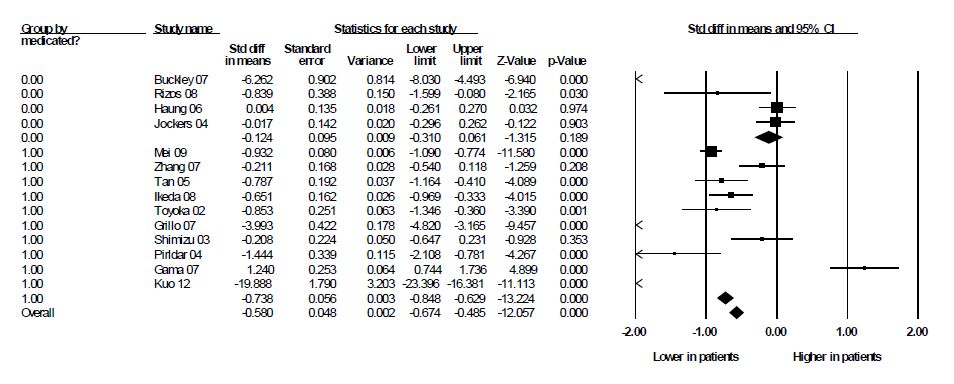
Buckley PF, Pillai A, Evans D, et al. (2007) Brain derived neurotrophic factor in first-episode psychosis. Schizophrenia Res 91: 1-5. doi: 10.1016/j.schres.2006.12.026
    [12] Grillo RW, Ottonin GL, Leke R, et al. (2007) Reduced serum BDNF levels in schizophrenic patients on clozapine or typical antipsychotics. J Psychiatric Res 41: 31-35. doi: 10.1016/j.jpsychires.2006.01.005
    [13] Gama CS, Andreazza AC, Kunz M, et al. (2007) Serum levels of brain-derived neurotrophic factor in patients with schizophrenia and bipolar disorder. Neurosci Letter 42: 45-48.
    [14] Mei HX, Hui L, Dang YF, et al. (2009) Decreased serum BDNF levels in chronic institutionalized schizophrenia on long term treatment with typical and atypical antipsychotics. Progress Neuropsychopharma Biol Psychiatry 33: 1508-1512. doi: 10.1016/j.pnpbp.2009.08.011
    [15] Zhang XY, Tan YL, Zhou DF, et al. (2007) Serum BDNF levels and weight gain in schizophrenic patients on long-term treatment with antipsychotics. J Psychiatric Res 41: 997-1004. doi: 10.1016/j.jpsychires.2006.08.007
    [16] Tan YL, Zhou DF, Cao LY, et al. (2005) Decreased BDNF in serum of patients with chronic schizophrenia on long-term treatment with antipsychotics. Neurosci Letter 382: 27-32. doi: 10.1016/j.neulet.2005.02.054
    [17] Ikeda Y, Yahata N, Ito I, et al. (2008) Low serum levels of brain-derived neurotrophic factor and epidermal growth factors in patients with chronic schizophrenia. Schizophrenia Res 101: 58-66. doi: 10.1016/j.schres.2008.01.017
    [18] Toyooka K, Asama K, Watanabe K, et al. (2002) Decreased levels of brain-derived neurotrophic factor in serum of chronic schizophrenic patients. Psychiatry Res 110: 249-257.
    [19] Rizos EN, Rontos I, Laskos E, et al. (2008) Investigation of serum BDNF levels in drug-naïve patients with schizophrenia. Progress Neuropsychopharma Biol Psychiatry 32: 1308-1311. doi: 10.1016/j.pnpbp.2008.04.007
    [20] Huang TL, Lee CT (2006) Associations between serum brain-derived neurotrophic factor levels and clinical phenotypes in schizophrenia patients. J Psychiatric Res 40: 664-668.
    [21] Shimizu E, Hashimoto K, Watanabe H, et al. (2003) Serum BDNF levels in schizophrenia are indistinguishable from controls. Neurosci Letters 351: 111-114. doi: 10.1016/j.neulet.2003.08.004
    [22] Pirildar S, Gönül AS, Taneli F, et al. (2004) Low serum levels of brain-deived neurotrophic factor in patients with schizophrenia do not elevate after antipsychotic treatment. Progress Neuropsychopharma Biol Psychiatry 28: 708-713.
    [23] Jockers-Scherübl MC, Danker-Hopfe H, Mahlberg R, et al. (2004) Brain-derived neurotrophic factor serum concentrations are increased in drug-naïve schizophrenic patients with chronic cannabis abuse and multiple substance abuse. Neurosci Letters 1: 79-83.
    [24] Kuo FC, Lee CH, Hsieh CH, et al. (2012) Lifestyle modification and behavior therapy effectively reduce body weight and increase serum level of brain-derived neurotrophic factor in obese non-diabetic patients with schizophrenia. Psychiatry Res 6.
    [25] Fatemi SH, Folsom TD (2009) The neurodevelopmental hypothesis of schizophrenia, revisited. Schizophrenia Bulletin 35: 528-548. doi: 10.1093/schbul/sbn187
    [26] Van de Kerkhoff NW, Fekkesa D, van der Heijden FMMA, et al. (2014) BDNF an S100B in psychotic disorders: evidence for and association with treatment responsiveness. Acta Neuropsychiatry 4: 223-229.
    [27] Rizos E, Papathanasiou MA, Michalopolu PG, et al. (2014) A longitudinal study of alterations of hippocampal volumes and serum BDNF levels in association to atypical antipsychotics in a sample of first episode patients with schizophrenia. PLoS One 9: e87997. doi: 10.1371/journal.pone.0087997
    [28] Gonzalez-Pinto A, Mosquera F, Palomini A, et al. (2010) Increase in brain-derived neurotrophic factor in first-episode psychotic patients after treatment with atypical antipsychotics. Int Clin Psychopharmacology 4: 241-245.
    [29] Durany N, Michel T, Zochling R, et al. (2001) Brain-derived neurotrophic factor and neurotrophin 3 in schizophrenic psychoses. Schizophrenia Res 52: 79-86.
    [30] Green MJ, Matheson SL, Shepherd A, et al. (2011) Brain-derived neurotrophic factor levels in schizophrenia: a systematic review with meta-analysis. Mol Psychiatry 16: 960-972. doi: 10.1038/mp.2010.88
    [31] Walker MP, la Ferla F, Salvador S, et al. (2013) Reversible epigenetic histone modifications and BDNF expression in neurons with aging and from a mouse model of Alzheimer's disease. AGE 35: 519-531. doi: 10.1007/s11357-011-9375-5
  • This article has been cited by:

    1. Santanu Bhattacharya, Nandadulal Bairagi, Regime shift and unbounded price in ecological–economic models: an interplay between harvesting and demand functions, 2025, 140, 2190-5444, 10.1140/epjp/s13360-025-06476-w
  • Reader Comments
  • © 2015 the Author(s), licensee AIMS Press. This is an open access article distributed under the terms of the Creative Commons Attribution License (http://creativecommons.org/licenses/by/4.0)
通讯作者: 陈斌, bchen63@163.com
  • 1. 

    沈阳化工大学材料科学与工程学院 沈阳 110142

  1. 本站搜索
  2. 百度学术搜索
  3. 万方数据库搜索
  4. CNKI搜索

Metrics

Article views(6189) PDF downloads(1278) Cited by(2)

Figures and Tables

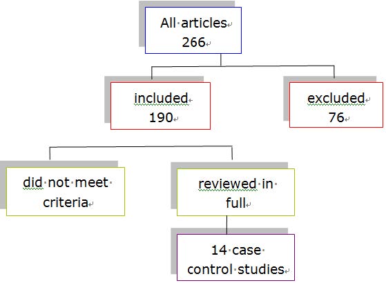
Figures(2)  /  Tables(3)

/

DownLoad:  Full-Size Img  PowerPoint
Return
Return

Catalog