
Citation: Jun He, Yan-Min Liu, Jun-Kang Tian, Ze-Rong Ren. A note on the inclusion sets for singular values[J]. AIMS Mathematics, 2017, 2(2): 315-321. doi: 10.3934/Math.2017.2.315
[1] | Mahmoud S. Mehany, Faizah D. Alanazi . An η-Hermitian solution to a two-sided matrix equation and a system of matrix equations over the skew-field of quaternions. AIMS Mathematics, 2025, 10(4): 7684-7705. doi: 10.3934/math.2025352 |
[2] | Vladislav N. Kovalnogov, Ruslan V. Fedorov, Denis A. Demidov, Malyoshina A. Malyoshina, Theodore E. Simos, Vasilios N. Katsikis, Spyridon D. Mourtas, Romanos D. Sahas . Zeroing neural networks for computing quaternion linear matrix equation with application to color restoration of images. AIMS Mathematics, 2023, 8(6): 14321-14339. doi: 10.3934/math.2023733 |
[3] | Kezheng Zuo, Yang Chen, Li Yuan . Further representations and computations of the generalized Moore-Penrose inverse. AIMS Mathematics, 2023, 8(10): 23442-23458. doi: 10.3934/math.20231191 |
[4] | Abdur Rehman, Ivan Kyrchei, Muhammad Zia Ur Rahman, Víctor Leiva, Cecilia Castro . Solvability and algorithm for Sylvester-type quaternion matrix equations with potential applications. AIMS Mathematics, 2024, 9(8): 19967-19996. doi: 10.3934/math.2024974 |
[5] | Wenxv Ding, Ying Li, Anli Wei, Zhihong Liu . Solving reduced biquaternion matrices equation k∑i=1AiXBi=C with special structure based on semi-tensor product of matrices. AIMS Mathematics, 2022, 7(3): 3258-3276. doi: 10.3934/math.2022181 |
[6] | Yang Chen, Kezheng Zuo, Zhimei Fu . New characterizations of the generalized Moore-Penrose inverse of matrices. AIMS Mathematics, 2022, 7(3): 4359-4375. doi: 10.3934/math.2022242 |
[7] | R. Sriraman, R. Samidurai, V. C. Amritha, G. Rachakit, Prasanalakshmi Balaji . System decomposition-based stability criteria for Takagi-Sugeno fuzzy uncertain stochastic delayed neural networks in quaternion field. AIMS Mathematics, 2023, 8(5): 11589-11616. doi: 10.3934/math.2023587 |
[8] | Qi Xiao, Jin Zhong . Characterizations and properties of hyper-dual Moore-Penrose generalized inverse. AIMS Mathematics, 2024, 9(12): 35125-35150. doi: 10.3934/math.20241670 |
[9] | Houssem Jerbi, Izzat Al-Darraji, Saleh Albadran, Sondess Ben Aoun, Theodore E. Simos, Spyridon D. Mourtas, Vasilios N. Katsikis . Solving quaternion nonsymmetric algebraic Riccati equations through zeroing neural networks. AIMS Mathematics, 2024, 9(3): 5794-5809. doi: 10.3934/math.2024281 |
[10] | R. Sriraman, P. Vignesh, V. C. Amritha, G. Rachakit, Prasanalakshmi Balaji . Direct quaternion method-based stability criteria for quaternion-valued Takagi-Sugeno fuzzy BAM delayed neural networks using quaternion-valued Wirtinger-based integral inequality. AIMS Mathematics, 2023, 8(5): 10486-10512. doi: 10.3934/math.2023532 |
In this article, we present an explicit spatially fourth-order accurate compact method for the Allen-Cahn (AC) equation [1,2] in one-, two-, and three-dimensional spaces. The AC equation is as follows:
∂ϕ(x,t)∂t=−F′(ϕ(x,t))ϵ2+Δϕ(x,t),x∈Ω,t>0, | (1.1) |
where the order parameter ϕ(x,t) is the difference of the local concentrations of the two components in a domain Ω, F(ϕ)=0.25(ϕ2−1)2 is a double well free energy density, and ϵ is a small parameter. The homogeneous Neumann boundary condition is assumed:
∂ϕ∂n=0on∂Ω, |
where ∂/∂n is the normal derivative on the boundary of domain. The AC equation (1.1) is L2-gradient flow of the Ginzburg–Landau functional:
E(ϕ)=∫Ω(F(ϕ)ϵ2+12|∇ϕ|2)dx. | (1.2) |
Developing high-order accurate numerical schemes is important, therefore, it has been widely studied. In studying high-order accurate numerical schemes in space, wide stencils are required. In this case, we should eliminate the inefficiency caused by calculating high-order derivatives with respect to space, such as the Laplace operator. Therefore, the compact scheme has been actively developed for high-order accurate schemes with relatively less wide stencils.
Abide [3] presented finite difference preconditioning for compact scheme discretizations of the Poisson equation with variable coefficients. Li and Liao [4] developed an explicit high-order compact finite difference method (FDM) to solve three-dimensional (3D) acoustic wave equations with spatially variable acoustic velocity. In [5], based on FDM, a high-order accurate compact method for the heat equation was studied on the inverse Lax-Wendroff boundary treatment. In [6], the authors developed a highly accurate local one-dimensional (1D) explicit compact method for the acoustic wave equation in two-dimensional (2D) space. Patel and Mehra [7] studied the fourth-order compact method for space fractional advection-diffusion reaction equations using the alternating direction implicit scheme. An explicit fourth-order compact scheme was developed for heat transfer of boundary layer flow [8], which has the advantage of finding solutions of nonlinear and linear convection-diffusion type equations that cannot be solved with the existing implicit compact scheme. Qiu et al. [9] developed a general conservative eighth-order compact finite difference method to solve the coupled Schrödinger-KdV equations, this method is decoupled and preserves several physical invariants in a discrete sense. Elmahdi and Huang [10] presented linearized finite difference and fourth-order compact finite difference schemes for the time fractional nonlinear diffusion-wave equations based on their equivalent partial integro-differential equations. Abdi et al. [11] presented high-order compact finite difference schemes for the fractional Black-Scholes equation in the case of European option pricing. Using implicit-type schemes, spatially fourth-order accurate compact schemes were presented in [12,13,14]. There are some studies for solving partial differential equation (PDE), including the Laplace terms using a fourth-order accurate method on hexagonal grids [15,16,17,18]. Zhai et al. [12] presented a linearized, temporally second-order, spatially fourth-order accurate compact method for the 3D AC equations with different boundary conditions. Long et al. [13] described the unconditional stable linear FDM for the 3D AC equation, combined with backward differentiation and fourth-order compact schemes. Bo et al. [14] theoretically proved the discrete maximum principle and energy stability of the compact difference scheme for AC equation in the 2D space and presented numerical examples. In [19], the authors presented a fourth-order FDM for the AC equation with a stabilized term which has an effect on structure-preserving.
Moreover, the compact finite difference scheme has been applied for solving the Cahn-Hilliard (CH) equation [20,21]:
∂ϕ(x,t)∂t=Δ(F′(ϕ)−ϵ2Δϕ), | (1.3) |
which is a phase-field model, H−1-gradient flow of the energy functional (1.2), modeling the phase separation of spinodal decomposition in a binary alloy. Li et al. [22] analyzed a three-level linearized compact method for the CH equation as proving the unique solvability and unconditional convergence of the numerical solution. Ju et al. [23] proposed a fast and stabilized compact exponential time differencing multi-step method for the CH equation. Lee [24] presented a fourth-order spatial and second-order temporal accurate, unconditionally stable compact FDM for the CH equation. Lee and Shin [25] presented a compact scheme for solving the CH equation with a periodic boundary condition. In [26], a fourth-order compact method for the pure stream function formulation of 3D unsteady incompressible Navier-Stokes equation was presented using the Crank-Nicolson method for time discretization.
Many studies for the compact scheme have adopted implicit-type schemes to numerically solve various equations. Implicit-type schemes have the advantage that they can solve the equations efficiently by using large time-step sizes compared to explicit-type schemes. On the other hand, in the case of a nonlinear partial differential equation, we need to use efficient numerical solvers such as multigrid methods. In addition, highly accurate results require small time-step sizes. For example, when we solve the CH equation which is a fourth-order nonlinear PDE, an explicit method imposes a severe constraint on time-step size for stability. A very small time-step size makes it almost impossible to compute the fine-grid solution. In this case, the multigrid method is useful. However, in this study, we focus on the fourth-order accurate compact method for the AC equation, which is a second-order nonlinear parabolic PDE. When we solve the AC equation using an explicit scheme, the linear term restricts the time-step size as Δt<0.5h2/d, where h is a mesh size and d is the spatial dimension [27,28,29]. The constraint on the time-step size is not too severe, therefore, the fourth-order compact explicit scheme increases the accuracy without greatly losing efficiency.
The main purpose of this study is to present a fully explicit spatially fourth-order accurate compact scheme for the AC equation in 1D, 2D, and 3D spaces. To the authors' knowledge, this is the first study of a fully explicit spatially fourth-order accurate compact scheme for the AC equation. The advantages of this study focusing on space are the accuracy and efficiency of the numerical solution, and the simplicity of implementation. In the follow-up study, we will improve the proposed scheme to be higher-order accuracy in time.
The layout of this paper is as follows. In Section 2, it is presented that the description of the fourth-order compact FDM for the AC equation. In Section 3, we perform various computational experiments to demonstrate the basic properties and advantages of the proposed method. Conclusions are made in Section 4.
Let Nx, Ny, and Nz be the number of grid points in the x, y, and z direction, respectively, Δt=T/Nt be the time-step size, T be the final time, and Nt be the total number of time steps.
In a 1D domain Ω=(ax,bx), let h=(bx−ax)/Nx be the uniform mesh size. A discrete numerical domain is denoted by Ωh={xi : xi=ax+(i−0.5)h, 1≤i≤Nx}. Let ϕni be the approximation of ϕ(xi,nΔt). The homogeneous Neumann boundary conditions for ϕ are given as follows: ϕ0=ϕ1,ϕ−1=ϕ2,ϕNx+1=ϕNx,ϕNx+2=ϕNx−1. The discrete differentiation operator is Dxϕi+12=(ϕi+1−ϕi)/h.
We discretize the AC equation in a 2D domain Ω=(ax,bx)×(ay,by). Let h=(bx−ax)/Nx=(by−ay)/Ny be the uniform mesh size. Let Ωh={(xi,yj) : xi=ax+(i−0.5)h, yj=ay+(j−0.5)h, 1≤i≤Nx, 1≤j≤Ny} be a discrete numerical domain. Let ϕnij be the approximation of ϕ(xi,yj,nΔt). The homogeneous Neumann boundary conditions for ϕ are given as follows:
for1≤j≤Ny,ϕ0,j=ϕ1,j,ϕ−1,j=ϕ2,j,ϕNx+1,j=ϕNx,j,ϕNx+2,j=ϕNx−1,j,for−1≤i≤Nx+2,ϕi,0=ϕi,1,ϕi,−1=ϕi,2,ϕi,Ny+1=ϕi,Ny,ϕi,Ny+2=ϕi,Ny−1. |
The discrete differentiation, gradient, and divergence operators are
Dxϕi+12,j=112ϕi+1,j+1−ϕi,j+1h+56ϕi+1,j−ϕijh+112ϕi+1,j−1−ϕi,j−1h,Dyϕi,j+12=112ϕi+1,j+1−ϕi+1,jh+56ϕi,j+1−ϕijh+112ϕi−1,j+1−ϕi−1,jh, |
∇cϕij=(Dxϕi+12,j,Dyϕi,j+12), and ∇d⋅(u,v)ij=(ui+12,j−ui−12,j)/h+(vi,j+12−vi,j−12)/h, respectively. The discrete l2-inner products and norms are defined as
(ϕ,ψ)h:=h2Nx∑i=1Ny∑j=1ϕijψij, | (2.1) |
(∇cϕ,∇cψ)e:=h2Nx∑i=1Ny∑j=1(Dxϕi+12,jDxψi+12,j+Dyϕi,j+12Dyψi,j+12), | (2.2) |
‖ϕ‖2=(ϕ,ϕ)h, and ‖∇ϕ‖2e=(∇cϕ,∇cϕ)e. | (2.3) |
We define the discrete total energy functional by
Eh(ϕn)=(F(ϕn),1)h+ϵ22‖∇ϕn‖2e, | (2.4) |
where 1 is a vector with all entries are 1.
We discretize the AC equation in a 3D domain Ω=(ax,bx)×(ay,by)×(az,bz). Let h=(bx−ax)/Nx=(by−ay)/Ny=(bz−az)/Nz and Ωh={(xi,yj,zk) : xi=ax+(i−0.5)h, yj=ay+(j−0.5)h, zk=az+(k−0.5)h, 1≤i≤Nx, 1≤j≤Ny, 1≤k≤Nz}. Let ϕnijk be the approximation of ϕ(xi,yj,zk,nΔt). The homogeneous Neumann boundary conditions for ϕ are given as follows:
for1≤j≤Ny,1≤k≤Nz,ϕ0jk=ϕ1jk,ϕ−1,jk=ϕ2jk,ϕNx+1,jk=ϕNx,jk,ϕNx+2,jk=ϕNx−1,jk,for−1≤i≤Nx+2,1≤k≤Nz,ϕi0k=ϕi1k,ϕi,−1,k=ϕi2k,ϕi,Ny+1,k=ϕi,Ny,k,ϕi,Ny+2,k=ϕi,Ny−1,k,for−1≤i≤Nx+2,−1≤j≤Ny+2,ϕij0=ϕij1,ϕij,−1=ϕij2,ϕij,Nz+1=ϕijNz,ϕij,Nz+2=ϕij,Nz−1. |
The discrete differentiation operators are
Dxϕi+12,jk=[128(ϕi+1,jk−ϕijk)+11(ϕi+1,j+1,k+ϕi+1,j−1,k+ϕi+1,j,k+1+ϕi+1,j,k−1−ϕi,j+1,k−ϕi,j−1,k−ϕij,k+1−ϕij,k−1)+2(ϕi+1,j+1,k+1+ϕi+1,j−1,k+1+ϕi+1,j+1,k−1+ϕi+1,j−1,k−1−ϕi,j+1,k+1−ϕi,j−1,k+1−ϕi,j+1,k−1−ϕi,j−1,k−1)]/(180h), |
and then Dyϕi,j+12,k and Dzϕij,k+12 are similarly defined above. We then define the discrete l2-inner products as
(ϕ,ψ)h:=h3Nx∑i=1Ny∑j=1Nz∑k=1ϕijkψijk, | (2.5) |
(∇cϕ,∇cψ)e:=h3Nx∑i=1Ny∑j=1Nz∑k=1(Dxϕi+12,jkDxψi+12,jk+Dyϕi,j+12,kDyψi,j+12,k+Dzϕij,k+12Dzψij,k+12). | (2.6) |
In a 1D space, a compact Laplace operator Δc is defined as follows:
Δcϕi=Δϕi=1h2(ϕi+1−2ϕi+ϕi−1). | (2.7) |
By the Taylor expansion, we can obtain
ϕ(x+Δx,t)=5∑k=0(Δx)kk!(∂∂x)kϕ(x,t)+O((Δx)6). | (2.8) |
Then, we can derive the following equation from Eq (2.8) by replacing Δx with ±h.
ϕ(x+h,t)−2ϕ(x,t)+ϕ(x−h,t)=h2ϕxx+h412ϕxxxx+O(h6). | (2.9) |
By dividing both sides of Eq (2.9) by h2, we obtain
Δcϕni=Δϕ(xi,tn)+h212Δ2ϕ(xi,tn)+O(h4), | (2.10) |
where Δ2ϕ=Δ(Δϕ) is the biharmonic operator. Note that the standard fourth-order 5-point Laplace operator Δs is defined as
Δsϕni=112h2(−ϕni−2+16ϕni−1−30ϕni+16ϕni+1−ϕni+2). |
From Eq (2.8), we can derive Δsϕi=Δϕ(xi)+O(h4) in the similar manner. Using Eq (2.10), we discretize the governing Eq (1.1) in a 1D domain as follows:
ϕn+1i−ϕniΔt+O(Δt)=−F′(ϕni)ϵ2+Δϕ(xi,tn)=−F′(ϕni)ϵ2+Δcϕni−h212Δ2ϕ(xi,tn)+O(h4)=−F′(ϕni)ϵ2+Δcϕni−h212Δ(∂ϕ(xi,tn)∂t+F′(ϕ(xi,tn))ϵ2)+O(h4)=−F′(ϕni)ϵ2+Δcϕni−h212(∂Δϕ(xi,tn)∂t+ΔF′(ϕ(xi,tn))ϵ2)+O(h4)=−F′(ϕni)ϵ2+Δcϕni−h212(∂Δcϕ(xi,tn)∂t+ΔcF′(ϕ(xi,tn))ϵ2+O(h2))+O(h4)=−F′(ϕni)ϵ2+Δcϕni−h212(Δcϕni−Δcϕn−1iΔt+O(Δt)+ΔcF′(ϕ(xi,tn))ϵ2)+O(h4). | (2.11) |
Therefore, up to O(Δt) and O(h4), we have
ϕn+1i−ϕniΔt=−F′(ϕni)ϵ2+Δcϕni−h212(Δcϕni−Δcϕn−1iΔt+ΔcF′(ϕni)ϵ2), | (2.12) |
for n≥2. Given ϕ0, ϕ1 is computed by using the standard fourth-order Laplacian Δs.
In a 2D space, the compact Laplace operator Δc [30] is defined as
Δcϕij=∇d⋅∇cϕij=16h2(ϕi−1,j+1+4ϕi,j+1+ϕi+1,j+1+4ϕi−1,j−20ϕij+4ϕi+1,j+ϕi−1,j−1+4ϕi,j−1+ϕi+1,j−1). |
By the Taylor series in two variables, we can obtain
ϕ(x+Δx,y+Δy)=5∑k=01k!(Δx∂∂x+Δy∂∂y)kϕ(x,y)+O((Δx)6+(Δy)6). |
By replacing Δx and Δy with different values ±h, we get
ϕ(x+h,y)+ϕ(x−h,y)+ϕ(x,y−h)+ϕ(x,y+h)=4ϕ+h2ϕxx+h2ϕyy+h412ϕxxxx+h412ϕyyyy+O(h6), | (2.13) |
ϕ(x−h,y−h)+ϕ(x−h,y+h)+ϕ(x+h,y−h)+ϕ(x+h,y+h)=4ϕ+2h2ϕxx+2h2ϕyy+h46ϕxxxx+h4ϕxxyy+h46ϕyyyy+O(h6). | (2.14) |
From Eqs (2.13) and (2.14), we have
ϕ(x−h,y−h)+ϕ(x−h,y+h)+ϕ(x+h,y−h)+ϕ(x+h,y+h)+4[ϕ(x+h,y)+ϕ(x−h,y)+ϕ(x,y−h)+ϕ(x,y+h)]−20ϕ(x,y)=6h2(ϕxx+ϕyy)(x,y)+h42(ϕxxxx+2ϕxxyy+ϕyyyy)(x,y)+O(h6). |
Finally, we have
Δcϕnij=Δϕ(xi,yj,tn)+h212Δ2ϕ(xi,yj,tn)+O(h4), | (2.15) |
where Δ2ϕ=Δ(Δϕ) is the biharmonic operator. Note that another standard fourth-order 9-point Laplace operator Δs is defined as
Δsϕnij=112h2(−ϕni−2,j+16ϕni−1,j−30ϕnij+16ϕni+1,j−ϕni+2,j)+112h2(−ϕni,j−2+16ϕni,j−1−30ϕnij+16ϕni,j+1−ϕni,j+2). |
In a similar way, Δsϕij=Δϕ(xi,yj)+O(h4). Figure 1 shows the nodes used by the compact and standard Laplace operators at a point, respectively.
Using Eq (2.15), similar to Eq (2.11), we discretize the governing Eq (1.1). Therefore, up to O(Δt) and O(h4), we have
ϕn+1ij−ϕnijΔt=−F′(ϕnij)ϵ2+Δcϕnij−h212(Δcϕnij−Δcϕn−1ijΔt+ΔcF′(ϕnij)ϵ2), | (2.16) |
for n≥2. Given ϕ0, ϕ1 is computed by using the standard fourth-order Laplacian Δs.
In a 3D space, a compact Laplace operator Δc [31] is defined as
Δcϕijk=∇d⋅∇cϕijk=130h2[14(ϕi+1,jk+ϕi−1,jk+ϕi,j+1,k+ϕi,j−1,k+ϕij,k+1+ϕij,k−1)+3(ϕi+1,j,k+1+ϕi+1,j,k−1+ϕi+1,j+1,k+ϕi+1,j−1,k+ϕi−1,j+1,k+ϕi−1,j−1,k+ϕi,j+1,k+1+ϕi,j−1,k−1+ϕi−1,j,k+1+ϕi−1,j,k−1+ϕi−1,j+1,k+1+ϕi−1,j−1,k−1+ϕi,j+1,k−1+ϕi,j−1,k+1)+ϕi−1,j+1,k−1+ϕi−1,j−1,k+1+ϕi+1,j+1,k+1+ϕi+1,j−1,k−1+ϕi+1,j+1,k−1+ϕi+1,j−1,k+1−128ϕijk]. |
By the Taylor expansion in three variables, we can obtain
ϕ(x+Δx,y+Δy,z+Δz,t)=5∑k=01k!(Δx∂∂x+Δy∂∂y+Δz∂∂z)kϕ(x,y,z,t)+O((Δx)6)+O((Δy)6)+O((Δz)6). | (2.17) |
Then, we can derive the following equations from Eq (2.17) by replacing Δx, Δy, and Δz with different values ±h.
ϕ(x+h,y,z,t)+ϕ(x−h,y,z,t)+ϕ(x,y+h,z,t)+ϕ(x,y−h,z,t)+ϕ(x,y,z+h,t)+ϕ(x,y,z−h,t)=6ϕ+h2(ϕxx+ϕyy+ϕzz)+h412(ϕxxxx+ϕyyyy+ϕzzzz)+O(h6), | (2.18) |
ϕ(x−h,y−h,z,t)+ϕ(x−h,y+h,z,t)+ϕ(x+h,y−h,z,t)+ϕ(x+h,y+h,z,t)+ϕ(x−h,y,z−h,t)+ϕ(x−h,y,z+h,t)+ϕ(x+h,y,z−h,t)+ϕ(x+h,y,z+h,t)+ϕ(x,y−h,z−h,t)+ϕ(x,y−h,z+h,t)+ϕ(x,y+h,z−h,t)+ϕ(x,y+h,z+h,t)=12ϕ+4h2(ϕxx+ϕyy+ϕzz)+h43(ϕxxxx+ϕyyyy+ϕzzzz)+h4(ϕxxyy+ϕyyzz+ϕxxzz)+O(h6), | (2.19) |
ϕ(x−h,y−h,z−h,t)+ϕ(x−h,y−h,z+h,t)+ϕ(x−h,y+h,z−h,t)+ϕ(x−h,y+h,z+h,t)+ϕ(x+h,y−h,z−h,t)+ϕ(x+h,y−h,z+h,t)+ϕ(x+h,y+h,z−h,t)+ϕ(x+h,y+h,z+h,t)=8ϕ+4h2(ϕxx+ϕyy+ϕzz)+h43(ϕxxxx+ϕyyyy+ϕzzzz)2h4(ϕxxyy+ϕyyzz+ϕxxzz)+O(h6). | (2.20) |
Multiplying both sides of Eqs (2.18)–(2.20) by 14, 3, and 1, respectively, and adding the equations, we have
30h2Δcϕijk=30h2(ϕxx+ϕyy+ϕzz)+52h4(ϕxxxx+ϕyyyy+ϕzzzz+2ϕxxyy+2ϕyyzz+2ϕxxzz)+O(h6). | (2.21) |
By dividing both the sides of Eq (2.21) by 30h2, we obtain
Δcϕnijk=Δϕ(xi,yj,zk,tn)+h212Δ2ϕ(xi,yj,zk,tn)+O(h4). | (2.22) |
Note that the 3D standard fourth-order 13-point Laplace operator Δs is defined as
Δsϕnijk=112h2(−ϕni−2,jk+16ϕni−1,jk−30ϕnijk+16ϕni+1,j−ϕni+2,j)+112h2(−ϕni,j−2,k+16ϕni,j−1,k−30ϕnijk+16ϕni,j+1,k−ϕni,j+2,k)+112h2(−ϕnij,k−2+16ϕnij,k−1−30ϕnijk+16ϕnij,k+1−ϕnij,k+2). |
In a similar way, Δsϕijk=Δϕ(xi,yj,zk)+O(h4). Figure 2 shows the grid point usages of standard Δh and compact Δh in a 3D space.
Using Eq (2.15), we discretize the governing Eq (1.1). Therefore, up to O(Δt) and O(h4), we have
ϕn+1ijk−ϕnijkΔt=−F′(ϕnijk)ϵ2+Δcϕnijk−h212(Δcϕnijk−Δcϕn−1ijkΔt+ΔcF′(ϕnijk)ϵ), | (2.23) |
for n≥2. Given ϕ0, ϕ1 is computed by using the standard fourth-order Laplacian Δs.
We demonstrate the representative properties of the explicit compact AC equation: phase separation, fourth-order accuracy in space, non-increase of total energy, and motion by mean curvature. We show the efficiency of our method using numerical comparison and measuring computational time. In addition, we perform the computational experiments for a non-convex initial condition with and without an obstacle to highlight the advantage of the proposed scheme. It can easily handle the computation on arbitrary complex domains.
We consider one of the most basic computational simulations, that is, the dynamics of phase separation. First, we conduct the numerical experiment in a 1D computational domain Ω=(0,1) with the initial condition given as
ϕ0i=0.1rand,for1≤i≤Nx, |
where rand is a random number in [−1,1]. To observe the equilibrium profile, we cease the iterative computation when the following criterion is met:
||ϕn−ϕn−1||2<1.0e-5, | (3.1) |
where n is a positive integer, and ϕn is called a numerical equilibrium solution. The parameters are taken as Nx=100,h=1/Nx,Δt=0.1h2, and ϵ=4h/(2√2tanh−1(0.9)). Figure 3 indicates the initial condition (t=0), numerical solution (t=30Δt), and numerical equilibrium solution (t=2242Δt). From this result, we can also numerically confirm that the numerical solutions are bounded between −1 and 1.
We next observe the phase separation in a 2D domain Ω=(0,1)2. The initial condition is given as
ϕ0ij=0.1rand,for1≤i≤Nx,1≤i≤Ny. | (3.2) |
The parameters are taken as Nx=Ny=100,h=1/Nx,Δt=0.1h2, and ϵ=4h/(2√2tanh−1(0.9)). Figure 4 indicates the initial condition (t=0) and numerical solutions (t=30Δt,100Δt). From this result, we can also numerically confirm that the numerical solutions are bounded between −1 and 1.
We investigate a quantitative estimate of the rate of convergence. Note that the discrete l2-norms of numerical solutions is defined as
||ϕn||2=√1NxNx∑i=1(ϕni)2,||ϕn||2=√1NxNyNx∑i=1Ny∑j=1(ϕnij)2, |
in 1D and 2D domains, respectively. First, in a 1D domain Ω=(0,2), we consider the traveling wave solution of the AC equation [32,33]:
ϕ(x,t)=12[1−tanh(x−0.7−st2√2ϵ)], | (3.3) |
where s=3ϵ/√2. At t=0, the initial profile is
ϕ(x,0)=12[1−tanh(x−0.72√2ϵ)]. | (3.4) |
Figure 5 shows the initial, numerical, and analytic profiles. Here, the parameters used are Nx=100,h=2/Nx,ϵ=8h/(2√2tanh−1(0.9)),Δt=0.1h2, and the final T=120Δt.
We perform a convergence test with the initial condition (3.4) on a set of increasingly finer mesh grid sizes. The computational solutions are computed on the uniform grids and time steps, h=2/Nx for Nx=40,80, and 160. The fixed time-step size is Δt=5.0e-9, the final time is T=50000Δt, and ϵ=0.025. The convergence rate is defined as the ratio of successive errors, that is, log2(||eNx||2/||e2Nx||2), where the discrete l2-norm error is defined as ||eNx||2=√1Nx∑Nxi=1(ϕ(xi,nΔt)−ϕni) and ||e2Nx||2=√12Nx∑2Nxi=1(ϕ(xi,nΔt)−ϕni). Table 1 lists the errors and rates of convergence and demonstrates that the proposed scheme is spatially fourth-order accurate.
h | 0.5000 | 0.0250 | 0.0125 | ||
l2-error | 1.6363e-4 | 9.8470e-6 | 6.2480e-7 | ||
Rate | 4.05 | 3.98 |
In a 2D domain Ω=(0,2)2, we consider the following solution:
ϕ(x,y,t)=12[1−tanh(0.8x+0.6y−0.88−st√2ϵ)]. | (3.5) |
The parameters are taken as N=Nx=Ny=100,h=2/N,Δt=0.1h2, ϵ=8h/(2√2tanh−1(0.9)), and the final time T=90Δt. In this test, the Dirichlet boundary condition is used and the values of order parameter on the boundary are set as the analytic solutions. Figures 6(a) and 6(b) show the initial profile at t=0 and the numerical solution at t=90Δt, respectively. Figure 6(c) shows the contours of the initial, numerical, and analytic solutions at the ϕ=0.5 level.
We conduct a convergence test with the initial condition (3.5) on a set of increasingly finer mesh grid sizes. The computational solutions are computed using h=2/N for N=40,80,160, the fixed time-step size Δt=1.0e-9, the final time T=250000Δt, and ϵ=0.025. Table 2 lists the errors and rates of convergence. Here, the discrete l2-norm error in a 2D domain is defined as ||eN||2=√1N2∑Ni=1∑Nj=1(ϕ(xi,yj,nΔt)−ϕnij). The results in the 2D domain suggest that the scheme is indeed fourth-order accurate in space.
h | 0.5000 | 0.0250 | 0.0125 | ||
l2-error | 9.3779e-5 | 6.2659e-6 | 3.9393e-7 | ||
Rate | 3.90 | 3.99 |
We verify that a numerical equilibrium solution in which the profile is a hyperbolic tangent is consistent with a theoretical solution when the time is large enough. The initial condition on a domain Ω=(−1,1) is
ϕ(x,0)=0.5tanh(x√2ϵ). | (3.6) |
The parameters are taken as Nx=200,h=2/Nx,Δt=0.1h2,t=5, and ϵ=4h/(2√2tanh−1(0.9)). In Figure 7, the numerical equilibrium profile agrees well with the analytic one
ϕ(x,t)=tanh(x√2ϵ). |
Here, the l2-norm error between two equilibrium profiles is less than 1.0e-16.
We numerically validate that the total energy functional (1.2) decreases over time. In a 2D domain, the discrete total energy is defined as
Eh(ϕn)=h2ϵ2Nx∑i=1Ny∑j=1F(ϕnij)+h22Nx∑i=1Ny∑j=1|∇cϕnij|2. |
The initial condition is defined as Eq (3.2) on Ω=(0,1)2. The parameters are used as follows: N=100,h=1/N,Δt=0.1h2,T=2000Δt, and ϵ=4h/(2√2tanh−1(0.9)). Figure 8 shows the time evolution of the discrete total energy and numerical solution. The normalized discrete total energy E(ϕn)/E(ϕ0) is non-increasing over time t. The snapshots of the numerical solutions are at t=0,0.002,0.006, and 0.02, respectively.
In this section, we verify the efficiency of the proposed method. First, we present numerical comparisons between the proposed scheme and previous work [13], and compare the performance using their computational time. In [13], the authors used the linear multigrid method to solve the AC equation using the fourth-order compact FDM. One V-cycle in the linear multigrid procedure consists of three parts: a pre-smoothing, a coarse grid correction, and a post-smoothing [34]. For the sake of convenience, we define the cost of performing one smoothing sweep on the finest grid as a work unit (WU). We assume that each number of pre- and post-smoothing sweeps is equal to the positive integer ν larger than 1. The smoothing steps mainly adopt the Gauss-Seidel type method, however, we apply the explicit method whose computational cost is less than that. The computational cost of the proposed method is estimated to be less than 2 WU, whereas that of the multigrid method in a 3D domain is
2ν(1+2−3+2−6+2−9+⋯+2−3N)<21−2−3νWU=16ν7WU, |
where N=Nx=Ny=Nz. In general, one V-cyle is not enough even though it depends on the given tolerance [35,36]. Hence, the computational cost of our method is estimated to be less than that of the multigrid method.
We use the initial condition as ϕ(x,y,z,0)=sin(2πx)sin(2πy)sin(2πz) on a domain Ω=(0,1)3, the mesh size N=32,64,128,256, and the other parameters as h=1/N,Δt=0.1h2,T=10Δt, and ϵ=0.1. Our computation is performed using MATLAB 2022b on an Intel Core i9-12900H CPU @ 2.50 GHz with 32 GB of RAM. We measure total CPU time (sec) for 10 time iterations and calculate it divided by the number of time iterations. Table 3 lists the average CPU times. Our method is more than 10 times faster than the implicit-type method.
Mesh size | 323 | 643 | 1283 | 2563 |
Long et al. [13] | 0.0373 | 0.2766 | 2.2953 | 17.8828 |
Ours | 0.0029 | 0.0201 | 0.1674 | 1.3946 |
Motion by mean curvature, the representative property of the AC equation, means that the interface Γ(t) of the solution evolves in the direction of the normal velocity proportional to the magnitude of the mean curvature [37]. The interface Γ(t) is defined by the zero-level set of the solution ϕ, i.e., Γ(t)={x∈Ω|ϕ(x,t)=0}. The normal velocity V of Γ(t) at each point x is
V(x,t)=−(κ1+κ2)=−(1R1+1R2), |
where κ1 and κ2 are the principal curvatures of the interface, and R1 and R2 are the principal radii. In this section, we only consider the case where the two principal radii are the same, therefore, we set the radius as R(t). In a 2D space, there is one principal radius, therefore, V=−1/R(t). In a 3D space, V=−2/R(t). Thus, for the spatial dimension d,
V=1−dR(t). | (3.7) |
Because the normal velocity V is the change in radius with time t,
V=dR(t)dt. | (3.8) |
From Eqs (3.7) and (3.8) and the initial radius R0=R(0), the analytic radius is
R(t)=√R20+2(1−d)t. |
For the details, refer to the references [37,38]. We demonstrate the motion by mean curvature in 2D and 3D domains. First, we perform a 2D simulation with the initial condition
ϕ(x,y,0)=tanh(R0−√(x−0.5)2+(y−0.5)2√2ϵ), |
in which the shape of zero-level contour is a circle with center (0.5,0.5) and radius R0=0.35, on Ω=(0,1)2. The parameters used are N=100,h=1/N,Δt=0.1h2,ϵ=4h/(2√2tanh−1(0.9)), and T=6000Δt. Figure 9(a) shows that the given circle shrinks in the direction of the normal vector according to motion by mean curvature. The zero-level contours are drawn every 600Δt from t=0 to t=6000Δt. From the contour spacing, it can be observed that the circle shrinks faster as the radius of the circle becomes smaller. Figure 9(b) indicates that the analytic and numerical radii agree with each other. Figure 9(c)–9(e) show the snapshots of the computational solution at time t=0,3600Δt, and 6000Δt, respectively.
We consider three circles with different centers and radii as shown in Figure 10(a). The initial condition is
ϕ(x,y,0)=tanh(0.27−√(x−0.35)2+(y−0.65)2√2ϵ)+tanh(0.17−√(x−0.72)2+(y−0.25)2√2ϵ)+tanh(0.1−√(x−0.8)2+(y−0.55)2√2ϵ)+2. |
Here, the parameters, N,h,ϵ,Δt, are used as described above. Figures 10(b) and 10(c) are the snapshots of the computational solutions at t=1200Δt and t=3000Δt, respectively. Figure 10(d) shows the zero-level contours every 300Δt from t=0 to t=3000Δt. The interface of the computational solution shrinks with the different velocities depending on the mean curvature of each circle. In other words, because the curvature of a circle with a smaller radius is large, the smaller-radius circle disappears first, and the larger-radius circle shrinks slowly.
Figure 11 shows the snapshots of the initial and numerical solution with the torus-type initial condition:
ϕ(x,y,0)=tanh(0.4−√(x−0.5)2+(y−0.5)2√2ϵ)−tanh(0.3−√(x−0.5)2+(y−0.5)2√2ϵ)−1, |
on Ω=(0,1)2. Here, the parameters, N,h,ϵ,Δt, are used as described above. In Figure 11, the top and bottom rows show mesh plots and zero-level contours of the solution, respectively, where the time t is 0,3000Δt, and 5000Δt. It is observed that the radius of the inner contour is smaller than that of the outer contour as shown in Figure 11. Hence, with motion by mean curvature, the inner contour decreases faster than the outer contour.
In addition, we observe the results of 2D simulation with the star-shaped initial condition on Ω=(0,1)2 as shown in Figure 12(a). We use N=150,h=1/N,Δt=0.1h2, and ϵ=8h/(2√2tanh−1(0.9)). Even though an initially complex shape is given, the part with the largest mean curvature is smoothed first, and then becomes circular. Figure 12(b) and 12(c) show mesh and contour plots of the computational solution at t=0,100Δt, and 3000Δt.
Next, we consider several computational simulations in a 3D domain to demonstrate motion by mean curvature. First of all, we verify the decreasing trend in the radius of a sphere. We conduct the 3D simulation with the following initial condition:
ϕ(x,y,z,0)=tanh(R0−√(x−0.5)2+(y−0.5)2+(z−0.5)2√2ϵ), |
i.e., a sphere with center (0.5,0.5,0.5) and radius R0=0.35, on the computational domain Ω=(0,1)3. The parameters used are N=Nx=Ny=Nz=80,h=1/N,Δt=0.1h2, and ϵ=4h/(2√2tanh−1(0.9)). Figure 13 shows that the given sphere shrinks in the direction of the normal vector according to motion by mean curvature.
Figure 14 shows the temporal evolution of a torus in a domain Ω=(0,1)×(0,1)×(0,0.5). The initial torus with center (0.5, 0.5, 0.25), large radius R1=0.25, and small radius R2=0.12 is defined as:
ϕ(x,y,z,0)=tanh(R2−√(R1−√(x−0.5)2+(y−0.5)2)2+(z−0.25)2√2ϵ). |
The parameters are used as Nx=Ny=100,Nz=50,h=0.01, ϵ=8h/(2√2tanh−1(0.9)),Δt=0.1h2, and T=700Δt.
On a computational domain Ω=(−1,1)3, we consider a sphere of center (0,0,0) and radius R0 perturbed by a spherical harmonic Yl,m [39,40]:
ϕ(x,y,z,0)=tanh(R0−√x2+y2+z2+AYl,m(θ,φ)√2ϵ), |
where A denotes amplitude, θ is the polar angle (measured from z-axis), and φ is the azimuthal angle (measured counterclockwise from the x-axis to the y-axis). Here, l=10,m=7,R0=0.7, and A=0.7. The parameters are used as N=100,h=2/N, ϵ=4h/(2√2tanh−1(0.9)),Δt=0.1h2, and T=1000Δt. Figure 15 shows the snapshots at t=0,200Δt, and 1000Δt. From the results, the temporal evolution works according to motion by mean curvature.
The implicit-type methods, compared to the explicit method, can use a relatively large Δt. However, it is difficult to implement their algorithms for the computational simulation. For example, the multigrid method is one of the most famous algorithms for solving implicitly discretized PDEs. If the computational domain is complex or there are obstacles that interfere with the evolution of order parameter ϕ, it gets more complicated. In contrast, our proposed explicit compact method can obtain the spatially fourth-order accurate solution for the AC equation efficiently even in complex domains or in the presence of obstacles. To demonstrate these advantages, we perform the computational simulations considering obstacles that are solid and fixed structures in 2D and 3D domains.
We use the non-convex initial condition and the rectangular bar-shaped obstacle in the 2D domain as shown in Figure 16(a). In Figure 16, from top to bottom, each row represents without the obstacle, with the obstacle, and overlapping the two cases. Here, the solid line and the purple area are the zero-level set of the solutions with and without the obstacle, respectively, and the green area inside the dotted line is the obstacle. The parameters used for the test are N=256, h=1/N, Δt=0.1h2, T=39000Δt, and ϵ=4h/(2√2tanh−1(0.9)) in the domain Ω=(0,1)2. The first row of Figure 16 shows the temporal evolution by mean curvature flow in the case without the obstacle as the numerical simulations presented in previous subsections. To perform the simulations with the obstacle, we perform iterative calculations for numerical solutions only at grid points in the whole domain except for obstacles. For the numerical solution near the obstacle, we always use the fixed solution, ϕ=−1, at points inside the obstacle. The second row of Figure 16 shows the temporal evolution of the zero-level set of numerical solutions with the obstacle. The mean curvature of the inward curves near the obstacle becomes larger than in the case without the obstacle. Therefore, the part with larger mean curvature, such as near the obstacle, shrinks faster according to motion by mean curvature. It is observed that the different mean curvature causes different results of temporal evolution depending on whether the obstacle exists as shown in the bottom row of Figure 16.
Next, we conduct the 3D experiments using the non-convex initial condition, where the values inside the surface are ϕ=1 and the outside is ϕ=−1 as shown in Figure 17(a). Figures 17(a)–17(d) illustrate the temporal evolutions of zero-level isosurface of the numerical solutions without and with the obstacle. In the second row of Figure 17, the green object represents the obstacle where the inside and boundary of the obstacle are fixed to ϕ=−1. Here, we use the numerical parameters as N=150, h=1/N, Δt=0.1h2, and ϵ=4h/(2√2tanh−1(0.9)) in the domain Ω=(0,1)3. Even in 3D space, the mean curvature of the area with the obstacle is maintained to be large, and the solution contracts faster than when there is no obstacle. The difference between 2D and 3D simulations is that there are two principal curvatures in the 3D domain, which complicates the analysis of the numerical results more than in the 2D cases. However, the basic mechanism is the same as the 2D simulations.
We presented the explicit spatially fourth-order accurate compact method for the AC equation. We use a fourth-order compact FDM, not only being more accurate but needing relatively less wide stencils for the discrete Laplace operator. The time step restriction that is the typical problem of the explicit Euler scheme is not severe because the governing equation is a second-order parabolic PDEs, and small temporal step sizes should be used for an accurate numerical solution. Moreover, it is simple to implement. Therefore, the proposed numerical algorithm is fast and efficient. We observed the phase separation phenomena using random number initial conditions, calculated the rate of convergence to verify the fourth-order accuracy in space, verified the hyperbolic tangent equilibrium profile, and numerically demonstrated the dissipation of discrete total energy. We verified the efficiency of the proposed method by comparing the computational cost between our method and the existing method. We performed various numerical simulations for motion by mean curvature, the representative property of the AC equation. Moreover, experiments comparing the numerical solutions with and without solid obstacles were performed to indicate that the proposed numerical algorithm is efficient and simple to implement. In previous research [41], the maximum bound principle and energy dissipation were proven for a one-step explicit method to the AC equation. On the other hand, this is a non-trivial and challenging task for the current proposed scheme, which involves a two-step method using the (n−1)-, n-, and (n+1)-th time step solutions. In this study, we focused on proposing a fully explicit fourth-order compact scheme and presenting numerical experiments of the proposed method for the AC equation. In future work, theoretical proof for the maximum bound principle, energy dissipation, and error estimates will be considered, drawing insights from the studies conducted by [42,43].
The authors declare they have not used Artificial Intelligence (AI) tools in the creation of this article.
The first author (C. Lee) was supported by the National Research Foundation of Korea (NRF) grant funded by the Korea government (MSIT) (No. 2022R1C1C2003896). The authors extend their thanks to the reviewers for the valuable and constructive input they provided during the revision of the article.
The authors declare there is no conflicts of interest.
[1] | L. Qi, Some simple estimates of singular values of a matrix, Linear Algebra Appl. 56 (1984), 105-119. |
[2] | L.L. Li, Estimation for matrix singular values, Comput. Math. Appl. 37 (1999), 9-15. |
[3] | R.A. Brualdi, Matrices, eigenvalues, and directed graphs, Linear Mutilinear Algebra, 11 (1982), 143-165. |
[4] | G. Golub, W. Kahan, Calculating the singular values and pseudo-inverse of a matrix, SIAM J. Numer. Anal. 2 (1965), 205-224. |
[5] | R.A. Horn, C.R. Johnson, Matrix Analysis, Cambridge University Press, Cambridge, 1985. |
[6] | R.A. Horn, C.R. Johnson, Topics in Matrix Analysis, Cambridge University Press, Cambridge, 1991. |
[7] | C.R. Johnson, A Geršgorin-type lower bound for the smallest singular value, Linear Algebra Appl., 112 (1989), 1-7. |
[8] | C.R. Johnson, T. Szulc, Further lower bounds for the smallest singular value, Linear Algebra Appl. 272 (1998), 169-179. |
[9] | W. Li, Q. Chang, Inclusion intervals of singular values and applications, Comput. Math. Appl., 45 (2003), 1637-1646. |
[10] | Hou-Biao Li, Ting-Zhu Huang, Hong Li, Inclusion sets for singular values, Linear Algebra Appl. 428 (2008), 2220-2235. |
[11] | R. S. Varga, Geršgorin and his circles, Springer Series in Computational Mathematics, Springer-Verlag, 2004. |
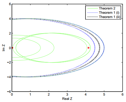
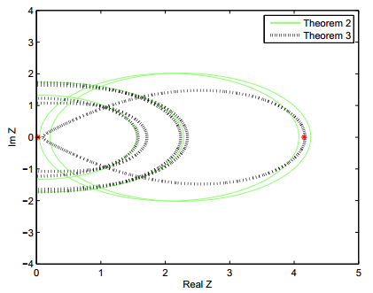
1. | Sondess B. Aoun, Nabil Derbel, Houssem Jerbi, Theodore E. Simos, Spyridon D. Mourtas, Vasilios N. Katsikis, A quaternion Sylvester equation solver through noise-resilient zeroing neural networks with application to control the SFM chaotic system, 2023, 8, 2473-6988, 27376, 10.3934/math.20231401 | |
2. | Houssem Jerbi, Obaid Alshammari, Sondess Ben Aoun, Mourad Kchaou, Theodore E. Simos, Spyridon D. Mourtas, Vasilios N. Katsikis, Hermitian Solutions of the Quaternion Algebraic Riccati Equations through Zeroing Neural Networks with Application to Quadrotor Control, 2023, 12, 2227-7390, 15, 10.3390/math12010015 | |
3. | Houssem Jerbi, Izzat Al-Darraji, Saleh Albadran, Sondess Ben Aoun, Theodore E. Simos, Spyridon D. Mourtas, Vasilios N. Katsikis, Solving quaternion nonsymmetric algebraic Riccati equations through zeroing neural networks, 2024, 9, 2473-6988, 5794, 10.3934/math.2024281 | |
4. | Spyridon D. Mourtas, P. Stanimirović, A. Stupina, I. Kovalev, Color restoration of images through high order zeroing neural networks, 2024, 59, 2271-2097, 01005, 10.1051/itmconf/20245901005 |
h | 0.5000 | 0.0250 | 0.0125 | ||
l2-error | 1.6363e-4 | 9.8470e-6 | 6.2480e-7 | ||
Rate | 4.05 | 3.98 |
h | 0.5000 | 0.0250 | 0.0125 | ||
l2-error | 9.3779e-5 | 6.2659e-6 | 3.9393e-7 | ||
Rate | 3.90 | 3.99 |
Mesh size | 323 | 643 | 1283 | 2563 |
Long et al. [13] | 0.0373 | 0.2766 | 2.2953 | 17.8828 |
Ours | 0.0029 | 0.0201 | 0.1674 | 1.3946 |
h | 0.5000 | 0.0250 | 0.0125 | ||
l2-error | 1.6363e-4 | 9.8470e-6 | 6.2480e-7 | ||
Rate | 4.05 | 3.98 |
h | 0.5000 | 0.0250 | 0.0125 | ||
l2-error | 9.3779e-5 | 6.2659e-6 | 3.9393e-7 | ||
Rate | 3.90 | 3.99 |
Mesh size | 323 | 643 | 1283 | 2563 |
Long et al. [13] | 0.0373 | 0.2766 | 2.2953 | 17.8828 |
Ours | 0.0029 | 0.0201 | 0.1674 | 1.3946 |