Processing math: 47%
Review Special Issues

A systematic review of the current state of collaborative mixed reality technologies: 2013–2018

  • Over the last few decades, Mixed Reality (MR) interfaces have received great attention from academia and industry. Although a considerable amount of research has already been done to support collaboration between users in MR, there is still no systematic review to determine the current state of collaborative MR applications. In this paper, collaborative MR studies published from 2013 to 2018 were reviewed. A total of 259 papers have been categorised based on their application areas, types of display devices used, collaboration setups, and user interaction and experience aspects. The primary contribution of this paper is to present a high-level overview of collaborative MR influence across several research disciplines. The achievements from each application area are summarised. In addition, remarkable papers in their respective areas are highlighted. Among other things, our study finds that there are three complementary factors to support and enhance collaboration in MR environments: (i) annotation techniques, which provide non-verbal communication cues to users, (ii) cooperative object manipulation techniques, which divide complex 3D object manipulation process into simpler tasks between different users, and (iii) user perception and cognition studies, which aim to lessen cognitive workload for task understanding and completion, and to increase users’ perceptual awareness and presence. Finally, this paper identifies research gaps and future directions that can be useful for researchers who want to explore ways on how to foster collaboration between users and to develop collaborative applications in MR.

    Citation: Ryan Anthony J. de Belen, Huyen Nguyen, Daniel Filonik, Dennis Del Favero, Tomasz Bednarz. A systematic review of the current state of collaborative mixed reality technologies: 2013–2018[J]. AIMS Electronics and Electrical Engineering, 2019, 3(2): 181-223. doi: 10.3934/ElectrEng.2019.2.181

    Related Papers:

    [1] Yitian Wang, Xiaoping Liu, Yuxuan Chen . Semilinear pseudo-parabolic equations on manifolds with conical singularities. Electronic Research Archive, 2021, 29(6): 3687-3720. doi: 10.3934/era.2021057
    [2] Yaning Li, Yuting Yang . The critical exponents for a semilinear fractional pseudo-parabolic equation with nonlinear memory in a bounded domain. Electronic Research Archive, 2023, 31(5): 2555-2567. doi: 10.3934/era.2023129
    [3] Mingyou Zhang, Qingsong Zhao, Yu Liu, Wenke Li . Finite time blow-up and global existence of solutions for semilinear parabolic equations with nonlinear dynamical boundary condition. Electronic Research Archive, 2020, 28(1): 369-381. doi: 10.3934/era.2020021
    [4] Jun Zhou . Initial boundary value problem for a inhomogeneous pseudo-parabolic equation. Electronic Research Archive, 2020, 28(1): 67-90. doi: 10.3934/era.2020005
    [5] Qianqian Zhu, Yaojun Ye, Shuting Chang . Blow-up upper and lower bounds for solutions of a class of higher order nonlinear pseudo-parabolic equations. Electronic Research Archive, 2024, 32(2): 945-961. doi: 10.3934/era.2024046
    [6] Fanqi Zeng, Wenli Geng, Ke An Liu, Boya Wang . Differential Harnack estimates for the semilinear parabolic equation with three exponents on Rn. Electronic Research Archive, 2025, 33(1): 142-157. doi: 10.3934/era.2025008
    [7] Yang Cao, Qiuting Zhao . Initial boundary value problem of a class of mixed pseudo-parabolic Kirchhoff equations. Electronic Research Archive, 2021, 29(6): 3833-3851. doi: 10.3934/era.2021064
    [8] Milena Dimova, Natalia Kolkovska, Nikolai Kutev . Global behavior of the solutions to nonlinear Klein-Gordon equation with critical initial energy. Electronic Research Archive, 2020, 28(2): 671-689. doi: 10.3934/era.2020035
    [9] Lianbing She, Nan Liu, Xin Li, Renhai Wang . Three types of weak pullback attractors for lattice pseudo-parabolic equations driven by locally Lipschitz noise. Electronic Research Archive, 2021, 29(5): 3097-3119. doi: 10.3934/era.2021028
    [10] Hui Yang, Futao Ma, Wenjie Gao, Yuzhu Han . Blow-up properties of solutions to a class of p-Kirchhoff evolution equations. Electronic Research Archive, 2022, 30(7): 2663-2680. doi: 10.3934/era.2022136
  • Over the last few decades, Mixed Reality (MR) interfaces have received great attention from academia and industry. Although a considerable amount of research has already been done to support collaboration between users in MR, there is still no systematic review to determine the current state of collaborative MR applications. In this paper, collaborative MR studies published from 2013 to 2018 were reviewed. A total of 259 papers have been categorised based on their application areas, types of display devices used, collaboration setups, and user interaction and experience aspects. The primary contribution of this paper is to present a high-level overview of collaborative MR influence across several research disciplines. The achievements from each application area are summarised. In addition, remarkable papers in their respective areas are highlighted. Among other things, our study finds that there are three complementary factors to support and enhance collaboration in MR environments: (i) annotation techniques, which provide non-verbal communication cues to users, (ii) cooperative object manipulation techniques, which divide complex 3D object manipulation process into simpler tasks between different users, and (iii) user perception and cognition studies, which aim to lessen cognitive workload for task understanding and completion, and to increase users’ perceptual awareness and presence. Finally, this paper identifies research gaps and future directions that can be useful for researchers who want to explore ways on how to foster collaboration between users and to develop collaborative applications in MR.


    In this paper, we consider the following initial boundary value problem of semilinear pseudo-parabolic equations with conical degeneration

    utΔButΔBu=|u|p1u, (xb,˜x)intB,t>0, (1.1)
    u(xb,˜x,0)=u0,                 (xb,˜x)intB, (1.2)
    u(0,˜x,t)=0,                    (0,˜x)B,t0, (1.3)

    where u0H1,n22,0(B), 1<p<n+2n2 and n=l+12 is the dimension of B, lN. Here the domain B=[0,1)×X is regarded as the local model near the conical singularity on conical singular manifolds, where XRl is a closed compact C manifold. Denoting the interior of B by intB and the boundary of B by B:={0}×X. We use the coordinates (xb,˜x):=(xb,x1,x2,...,xl)B for 0xb<1, ˜xX near B. The conical Laplacian operator is defined as

    ΔB=2B=(xbxb)2+2x1+...+2xl,

    which is the totally characteristic degeneracy operators on a stretched conical manifold, and B=(xbxb,x1,...,xl) denotes the corresponding gradient operator with conical degeneracy on the boundary B. In particular, we intend to investigate problem (1.1)-(1.3) in the weighted Mellin-Sobolev spaces H1,n22,0(B), and the definition of such distribution spaces will be introduced in Section 2.

    The classical pseudo-parabolic equation

    utΔutΔu=|u|p1u, xΩ,t>0, (1.4)

    defined on a bounded domain ΩRn with smooth boundary appeared in various physical and biological phenomena. For example, taking u as the flow velocity, the homogeneous form of the model equation (1.4) was introduced to study the incompressible simple fluids with fading memory and the non-steady flow with the Rivlin-Ericksen tensors [47,16]. One can also know more about other applications by referring to [23,24,5].

    It is well known that equation (1.4) in the domains contained in classical Euclidean space with regular boundary has been well investigated. Cao et al. [9] considered the Cauchy problem of following model

    tukΔut=Δu+up, xRn,t>0,

    and obtained the critical global existence exponent and the critical Fujita exponent by integral representation and contraction mapping principle. Subsequently, its uniqueness was proved by Khomrutai in [27] for the case 0<p<1. Furthermore, Li and Du [32] considered the Cauchy problem of

    utkΔut=Δu+|x|σup, xRn,t>0,

    and achieved the global existence and blowup in finite time of solutions with the critical Fujita exponent and the second critical exponent respectively. They also showed that the inhomogeneous term |x|σ affects the decay asymptotic behavior of solutions and accelerates the blowup of solutions. Khomrutai [28] studied the Cauchy problem of sublinear pseudo-parabolic equation

    tuΔtu=Δu+V(x,t)up, xRn,t>0,

    where V(x,t)λ(t)|x|σ is a non-autonomous and unbounded potential function with 0<p<1, and established the global existence of solutions by approximation and monotonicity argument. They also derived the precise grow-up rate of solutions and critical growth exponent. In order to figure out the effects of small perturbation on the dynamical of diffusion and reaction, Cao and Yin [8] considered the following Cauchy problem

    tukΔut=Δu+up+f(x), xRn,t>0,

    and revealed that small perturbation may develop large variation of solutions as time evolves. We also recommend that the reader refer to [43] to learn more about the effects of the power index of nonlinearity on the dynamical behavior of the solution. Different from above studies that focus on the influence of the nonlinearities especially the power index on the global well-posedness of the solution, [50,49,36] comprehensively studied equation (1.4) by considering the influences of the initial data on the global well-posedness and corresponding properties of solution. Depending on the potential well depth, they classified the initial data to subcritical initial energy level J(u0)<d, critical initial energy level J(u0)=d and supcritical initial energy level J(u0)>d, and proved the global existence, finite time blow up and asymptotic behavior of solutions with J(u0)d. Moreover, thanks to the comparison principle, the global existence and nonexistence of solutions were also obtained at supcritical initial energy level J(u0)>d. When the nonlinear effects are dominated by the logarithmic term, Chen [14] investigated the following nonlinear pseudo-parabolic equation, i.e.,

    tuΔuΔtu=uln|u|, xΩ,t>0

    and proved the global existence and the finite time blow up of solutions under the subcritical and critical initial energy case, respectively. Focusing on the high initial energy level, Xu and Wang et al [51] studied the problem proposed in [50] and gave a sufficient condition on initial data leading to blow up in finite time by the potential well method, at the same time, they also estimated the upper bound of the blowup time. As an important method to reveal the influence of initial data on the dynamical behavior of solutions, the potential well theory can be applied not only to the study of the problem of parabolic equations, but also to the study of the problem for various types of nonlinear evolution equations or systems. Xu and Lian et al [48] investigated the global well-posedness of solutions for coupled parabolic systems in the variational framework, and the initial data leading to the global existence or finite time blow up of the solution are divided. Chen and Xu [15] considered a class of damped fourth-order nonlinear wave equations with logarithmic sources. By examining the effect of weak nonlinear sources on the blow up of the solution, they revealed the confrontation mechanism between the damping structure and the nonlinear source and found the initial data that caused the solution to blow up in infinite time. For related results of polynomial nonlinear sources, we refer to [52]. Furthermore, we suggest the readers refer to [53] for the study of high order nonlinear wave equations, [54,34] for the study of damped nonlinear wave equation problems using improved potential well methods at high initial energy levels, and so on, which are representative recent results, of course we can not list all of the results obtained by the potential well theory here due to the huge amount.

    Actually, geometric singularities have attracted considerable interest and have become the focus of extensive physical and mathematical research in recent years. To find static solutions of Einstein's equations coupled to brane sources, Michele [39] studied the generalizations of the so-called "football" shaped extra dimensions scenario to include two codimension branes, which can be transformed into the mathematical problem of solving the Liouville equation with singularities, where the function space he constructed can be described as a sphere with conical singularities at the brane locations. After that some cone solitons (in the case of compact surfaces) were found by Hamilton [25], where cone singularities also arise naturally on the study of such kind of solitons. Not only being widely applied in cosmology and physics, the cone singular manifold itself also brings a lot of interesting topics to pure mathematics, such as the analytic proof of the cobordism theorem [31]. Conical singularities become a hotspot mainly for reasons of two aspects. Firstly, a manifold with conical singularities is one of the most fundamental stratified spaces and the investigation on it is motivated by the desire of understanding the dynamic behavior of the solution of nonlinear evolution equations on such stratified space. Topologically these spaces are of iterated cone type, in which, due to the conical singularity, the classical differential operator cannot be applied to such manifolds. Secondly, the methods developed for the domains with smooth boundaries cannot be directly applied to domains with singularities. It is a challenge and also an interesting problem in the community to restitute the conclusions established on the smooth domain for the problems defined on the conical space.

    Inspired by above, it is natural to bring some ideas and develop techniques to establish a comprehensive understanding of operator theory on the manifolds with conical singularities, which was first explored by Kondrat'ev in [29] by introducing the celebrated Mellin-Sobolev spaces Hs,γp(B) as the work space for the partial differential equations, then the theory on the conically degenerate pseudo-differential operator and the weighted Sobolev space on the conical manifolds were summarized by Schulze and Egorov in [45] and [18]. With the development of the study related to the singularity problem, including the study on the partial differential equation on manifolds with conical singularities, there occurs a large number of related results about various kinds of initial boundary value problems for evolution equations. For example, when using the porous medium equation to describe the flow of a substance in a porous medium material, the medium usually shows various irregular shapes in different regions, among which the most essential case is that the boundary of region includes the conical singularities. In order to discuss such situation for the porous medium equation, Lian and Liu [33] studied the initial-boundary value problem of the porous medium equation

    ut=Δum+V(x)up, xD,t>0

    in a cone D=(0,)×Sn1, and they proved that if the nonlinear power index p belongs to a suitable interval then the problem has no global non-negative solutions for any non-negative initial datum u0 unless u00. Beside that, they also showed that this problem has global solutions for some u00 when the nonlinear power index p is out of that interval. Considering the following porous medium equation

    utΔum=f(u,t), xD,t>0 (1.5)

    Roidos and Schrohe [44] obtained some results about the existence, uniqueness and maximal Lp-regularity of a short time solution and showed the short time asymptotic behavior of the solution near the conical point. In addition, the behavior for large times of non-negative solutions to the linear Dirichlet problem of equation (1.5) in cone-like domains was obtained by Andreucci [2]. For more related work, we refer to Laptev [19,30] for the high-order evolution inequalities in cone-like domains and Mazzeo et al [38] for the Ricci flow on asymptotically conical surfaces.

    As a differential operator reflecting the diffusion form on the conical singular manifold, the emergence of the cone operator ΔB brings about the first problem that needs to be solved urgently is the existence of solution of the differential equation. Unlike the usual smooth domain, the appearance of cone singularities makes the classical embedding theorem fail, which baffles the proof of the existence theorem. Therefore, in order to overcome the difficulty and obtain the existence of the weak solution by variational method in H1,n22,0(B), Chen et al [12] considered the nonlinear Dirichlet boundary value problems on manifolds with conical singularities

    ΔBu=|u|p1u, xintB,

    and obtained the existence of non-trivial weak solution. Moreover, they also established the well-known cone Sobolev inequality and Poincarˊe inequality in the weighted Sobolev spaces. Subsequently, Chen et al [13] extended this result to the nonlinear elliptic equations with a general nonlinear source and the critical Sobolev exponents respectively. These works describe the mechanism by which cone differential operators act on the regularity of solutions of differential equations. Of course, differential operators do more than affect the regularity of solutions. The influence of degenerate differential operators on the solutions of nonlinear elliptic equations is also reflected in many other aspects such as the eigenvalue problems and the existence of multiple solutions. Far from being complete, we refer the readers to [22,42,40,41,3] and references therein. It is worth to mention here that the change of the variational structure of equations caused by the non-classical forms of differential operators can bring big challenges to the application of variational techniques [21,7]. Further more, when utilizing the variational techniques the geometrical feature needs to be taken into consideration [20]. In fact we need to overcome the difficulties mentioned above in the application of variational techniques to the parabolic version.

    In order to understand the effect of different initial data belonging to H1,n22,0(B) on the well-posedness of the solution, Chen and Liu [11] investigated the following conical degenerate parabolic equation on the conical manifold

    utΔBu=|u|p1u, xintB,t>0,

    and obtained not only the existence of global solutions with exponential decay, but also the blow up in finite time under low initial energy level and critical initial energy level. Recently, Mohsen and Morteza [1] studied the semilinear conical-degenerate parabolic equation

    tuΔBu+V(x)u=g(x)|u|p1u, xintB,t>0,

    where V(x)L(intB)C(intB) is the positive potential function and gL(intB)C(intB) is a non-negative weighted function. Then they got the results of global solutions with exponential decay and showed the finite time blow up of solutions on manifolds with conical singularities under subcritical initial energy level J(u0)<d.

    Our goal is to obtian local and global well-posedness of solutions to problem (1.1)-(1.3). In details, by the potential well method, we classify the initial datum and give a threshold condition, which tells us that as long as the initial datum falls into the specified invariant set and the initial energy satisfies J(u0)d, the solution exists as a global one or blow up in a finite time. Moreover, for global solutions, we give an estimation of the asymptotic behavior of them. For the solution that blows up in finite time, we estimate the lower bound of the blowup time. Different from previous proofs in the potential well framework, we integrate the proofs of the sub-critical and critical initial energy cases as a whole part, which makes the results much more concise. Last but not least, we also investigate the finite time blow up of solutions to problem (1.1)-(1.3) at high initial energy levels. By giving a sufficient condition tied to the initial data in weighted Sobolev space H1,n22,0(B), the theorem can not only explain what kind of initial data cause the solution to blow up in finite time, but also get the corresponding upper bound estimate of the blowup time.

    The content of this paper is arranged as follows. In Section 2, we give the geometric description of conical singularities, the definitions of the weighted Sobolev spaces and several propositions of the manifold with conical singularities. Then we introduce the potential well structure for problem (1.1)-(1.3) and prove a series of corresponding properties in Section 3. Section 4 is concerned with the local existence and uniqueness theory. In Section 5, we not only prove the invariant manifolds, global existence and decay of solutions to describe the corresponding asymptotic behavior, but also prove the finite time blow up of solutions and estimate the lower bound of blowup time in Theorem 5.2. In Section 6, we give a sufficient condition to obtain the finite time blow up of the solution in Theorem 6.4. In particular, we also estimate the upper bound of the blowup time of the solution. Finally, some remarks and acknowledgements about this paper are given.

    In this section, main definitions of the manifold with conical singularities together with a brief description of its properties are given, for more details we refer to [45,18] and the references therein. Furthermore, we introduce some functional inequalities on the manifold with conical singularity, for more applications of these inequalities one can refer to [12,13].

    For l2, let XSl be a bounded open set in a unit sphere of R1+lˆx, and define the straight cone XΔ by

    XΔ={ˆxR1+l | ˆx=0 or ˆx|ˆx|X}.

    The polar coordinates (ρ,θ) gives us a description of XΔ{0} in the form X=R+×X, which is called the open stretched cone with the base X, and {0}×X is the boundary of X.

    Now we extend it to a more general situation by describing the singular space associated with a manifold with conical singularities. A finite dimensional manifold B with finite conical singularities B0={b1,b2,...,bN} has the following two properties:

    a) BB0 is a C manifold.

    b) Any biB0 (i=1,2,...,N) has an open neighborhood G in B, such that there is a homeomorphism χ:GXΔ for some closed compact C manifold X=X(bi), and φ restricts a diffeomorphism φ:G{0}X.

    By above assumptions we can define the stretched manifold associated with B. Let B be a C manifold with compact C boundary BbiB0X=X(bi) for which there exists a diffeomorphism

    BB0BB:=intB.

    Furthermore, the restriction of this diffeomorphism to Gibi is also a diffeomorphism GibiUiX(bi), where GiB is an open neighborhood near bi, and UiB is a collar neiborhood with Ui[0,1)×X(bi).

    The typical differential operators on a manifold with conical singularities, i.e., the so-called Fuchsian type operators in a neighborhood of xb=0, have the following form

    A:=xμbμk=0ak(xb)(xbxb)k

    with (xb,˜x)X and ak(xb)C(¯R+,Diffμk(X))[45,18]. For such singular operators, we introduce the following cone weighted Sobolev space.

    Definition 2.1 (The space Hm,γp(Rn+)). For (xb,˜x)R+×Rl:=Rn+, mN, γR and 1<p<, assume u(xb,˜x)D(Rn+), where the dual (C0(Rn+))=D(Rn+) is the space of all distributions in Rn+. We denote the spaces

    Hm,γp(Rn+):={uD(Rn+) | xNpγb(xbxb)kα˜xuLp(Rn+)}

    for any kN, multi-index αNn with k+|α|m.

    Therefore, Hm,γp(Rn+) is a Banach space with the following norm

    uHm,γp(Rn+)=k+|α|m(R+RNxNb|xγb(xbxb)kα˜xu(xb,˜x)|pdxbxbd˜x)1p.

    Definition 2.2 ([45] The space Hm,γp,0(B)). We give the definition of Hm,γp,0(B) as follows

    (ⅰ) Let X be a closed compact C manifold covered by open neighborhoods O={O1,...,ON} of the coordinate. Let the subordinate partition of unity {ψ1,...,ψN} be fixed and charts χj:OjRn, j=1,...,N. Then we say that uHm,γp(X) if and only if uD(X), whose norm is defined as follows

    uHm,γp(X)=(Nj=1(1×χj)1ψjupHm,γp(Rn+))1p,

    where 1×χj:C0(R+×Rn)C0(R+×Oj) is the pull-back function with respect to 1×χj:R+×OjR+×Rn. And the closure of C0(X) in Hm,γp(X) is denoted as Hm,γp,0(X).

    (ⅱ) Let B be the stretched cone manifolds. Then Hm,γp(B) denotes the subspace of all uWm,ploc(intB) such that

    Hm,γp(B)={uWm,ploc(intB) | ωuHm,γp,0(X)}

    for any cut-off function ω(xb) supported by a collar neighborhood of xb(0,1). Moreover, the subspace Hm,γp,0(B) of Hm,γp(B) is defined as follows

    Hm,γp,0(B)=[ω]Hm,γp,0(X)+[1ω]Wm,p0(intB),

    where the classical Sobolev space Wm,p0(intB) denotes the closure of C0(intB) in Wm,p(˜B) for ˜B as a closed compact C manifold of dimension n containing B as a submanifold with boundary.

    Proposition 1 (Cone Sobolev inequality [12]). Assuming 1p<n,  1p=1p1n then for all u(xb,˜x)C0(Rn+) the following estimate

    uLγp(Rn+)c1(xbxb)uLγp(Rn+)+(c1+c2)ni=1xiuLγp(Rn+)+c2c3uLγp(Rn+) (2.1)

    holds, where γ,γR are constants with γ=γ1, and

    c1=(n1)pn(np),
    c2=(n1)p|(n1)(γ1)(n1)pnp|1nn(np)

    and

    c3=(n1)pnp.

    Moreover, for u(xb,˜x)H1,γp,0(Rn+), there holds

    uLγp(Rn+)CuH1,γp,0(Rn+),

    where C=c1+c2.

    Proposition 2 (Cone Poincarˊe inequality [12]). Let B=[0,1)×XRn+ is bounded and 1<p<, γ is a constant. If u(xb,˜x)H1,γp,0(B) then

    u(xb,˜x)Lγp(B)cBu(xb,˜x)Lγp(B),

    where the optimal constant c depends only on B and p.

    Proposition 3 (Cone Hölder inequality [13]). If uLnpp(B),vLnpp(B) with p,p(1,) and 1p+1p=1, then we have the following cone type Hölder inequality

    B|uv|dxbxbd˜x(B|u|pdxbxbd˜x)1p(B|v|pdxbxbd˜x)1p.

    Proposition 4 (Eigenvalue problem [13]). There exist 0<λ1<λ2λ3...λk..., such that for each k1, the following Dirichlet problem

    {ΔBψk=λkψk,  (xb,˜x)intB,ψk=0,  (xb,˜x)B,

    admits a non-trivial solution in H1,n22,0(B). Moreover, {ψk}k1 constitute an orthonormal basis of the Hilbert space H1,n22,0(B).

    In order to state our main results, we shall introduce some definitions and notations as follows. In the sequel, for convenience we denote

    (u,v)B=Buvdxbxbd˜x   and   uLnpp(B)=(B|u|pdxbxbd˜x)1p.

    Furthermore, we denote H1,n22,0(B):=((B,B)B+(,)B)12. Of course, the norm H1,n22,0(B) is equivalent to the norm Ln22(B), which can be stemmed from Proposition 2.

    Throughout the paper, C will be used to denote various positive constants, whose value may change from line to line, and its dependence on other variables will be emphasised only if needed.

    Definition 3.1. (Weak solution). A function u is called a weak solution to problem (1.1)-(1.3) on [0,T]×B, if it satisfies

    (ⅰ) uL(0,T;H1,n22,0(B)) and utL2(0,T;H1,n22,0(B));

    (ⅱ) u(0)=u0;

    (ⅲ) for any ηH1,n22,0(B), the identity

    But(t)ηdxbxbd˜x+BBut(t)Bηdxbxbd˜x+BBu(t)Bηdxbxbd˜x
    =B|u(t)|p1u(t)ηdxbxbd˜x

    holds for a.e. t[0,T].

    Let us introduce the following functionals on the cone Sobolev space H1,n22,0(B) as the potential energy functional

    J(u)=12B|Bu|2dxbxbd˜x1p+1B|u|p+1dxbxbd˜x (3.1)

    and the so-called Nehari functional

    I(u)=B|Bu|2dxbxbd˜xB|u|p+1dxbxbd˜x. (3.2)

    Then J(u) and I(u) are well-defined and belong to C1(H1,N22,0(B),R).

    The weak solution u(t) in Definition 3.1 satisfies the conservation of energy, i.e.,

    t0ut(τ)2H1,n22,0(B)dτ+J(u(t))=J(u0),   0t<T. (3.3)

    By making use of the functionals above, we define the potential well depth d as follows

    d=infuNJ(u)>0, (3.4)

    where the Nehari manifold

    N={uH1,n22,0(B) | I(u(t))=0,B|Bu(t)|2dxbxbd˜x0} (3.5)

    separates the whole space H1,n22,0(B) into the following two unbounded manifolds

    N+={uH1,n22,0(B) | I(u(t))>0} (3.6)

    and

    N={uH1,n22,0(B) | I(u(t))<0}. (3.7)

    Furthermore, we introduce the following potential well

    W:=N+{0} (3.8)

    and the outside of the corresponding potential well

    V:=N. (3.9)

    Now, we give some corresponding properties of the potential well as follows.

    Lemma 3.2 (The properties of the energy functional J(u)). Assume that uH1,n22,0(B) and BuLn22(B)0, we have

    (i) limλ0j(λ)=0 and limλ+j(λ)=, where j(λ):=J(λu);

    (ii) there exist a unique λ=λ(u)>0, such that j(λ)=0;

    (iii) j(λ) is strictly increasing on 0λ<λ, strictly decreasing on λ>λ and takes the maximum at λ=λ;

    (iv) i(λ)>0 for 0λ<λ, i(λ)<0 for λ>λ and i(λ)=0, where i(λ):=I(λu).

    Proof. (ⅰ) From the definition of J(u), we know that

    j(λ)=J(λu)=λ22B|Bu|2dxbxbd˜xλp+1p+1B|u|p+1dxbxbd˜x,

    which gives limλ0j(λ)=0 and limλ+j(λ)=.

    (ⅱ) An easy calculation shows that

    j(λ)=λ(B|Bu|2dxbxbd˜xλp1B|u|p+1dxbxbd˜x). (3.10)

    Then taking j(λ)=0 we obtain that

    λ=(B|Bu|2dxbxbd˜xB|u|p+1dxbxbd˜x)1p1>0.

    (ⅲ) By a direct calculation, (3.10) gives j(λ)>0, for 0<λ<λ, j(λ)<0 for λ<λ<. Hence, the conclusion of (ⅲ) holds.

    (ⅳ) The conclusion follows from

    i(λ)=I(λu)=λ2B|Bu|2dxbxbd˜xλp+1B|u|p+1dxbxbd˜x=λj(λ).

    Next we give the relationship between uH1,n22,0(B) and I(u) in the following lemma.

    Lemma 3.3 (The properties of the Nehari functional I(u)). Suppose that uH1,n22,0(B) and r=(1(c2+1)Cp+1)1p1, where c and C are the optimal constants of the cone Poincarˊe inequality and cone Sobolev inequality respectively.

    (i) If 0<uH1,n22,0(B)<r, then I(u)>0.

    (ii) If I(u)<0, then uH1,n22,0(B)>r.

    (iii) If I(u)=0, then uH1,n22,0(B)r or uH1,n22,0(B)=0.

    Proof. (ⅰ) From 0<uH1,n22,0(B)<r, we have

    B|u|p+1dxbxbd˜xCp+1up+1H1,n22,0(B)<Cp+1rp1u2H1,n22,0(B)=1c2+1u2H1,n22,0(B)Bu2Ln22(B).

    Then by the definitions of r and I(u) we obtain that I(u)>0.

    (ⅱ) It is easy to see that uH1,n22,0(B)0 by I(u)<0. Combining cone Poincarˊe inequality and cone Sobolev inequality, it follows that

    u2H1,n22,0(B)=B|Bu|2dxbxbd˜x+B|u|2dxbxbd˜x(c2+1)B|Bu|2dxbxbd˜x<(c2+1)B|u|p+1dxbxbd˜x(c2+1)Cp+1up+1H1,n22,0(B),

    then we get

    uH1,n22,0(B)>(1(c2+1)Cp+1)1p1=r.

    (ⅲ) If I(u)=0 and uH1,n22,0(B)0, then by

    u2H1,n22,0(B)=B|Bu|2dxbxbd˜x+B|u|2dxbxbd˜x(c2+1)B|Bu|2dxbxbd˜x=(c2+1)B|u|p+1dxbxbd˜x(c2+1)Cp+1up+1H1,n22,0(B),

    we get uH1,n22,0(B)(1(c2+1)Cp+1)1p1=r.

    The depth d can be estimated as follows.

    Lemma 3.4 (The potential well depth). Suppose that 1<p<n+2n2 and d is defined as (3.4). Then we have

    d=infuNJ(u)=p12(p+1)(1(c2+1)p+12Cp+1)2p1, (3.11)

    where c is the best coefficient of the cone Poincarˊe inequality.

    Proof. Suppose that uN, then uH1,n22,0(B)r from Lemma 3.3. Thus according to the definition of J(u), I(u) and cone Poincarˊe inequality, we arrive at

    J(u)=(121p+1)B|Bu|2dxbxbd˜x+1p+1I(u)(121p+1)1c2+1u2H1,n22,0(B)p12(p+1)(c2+1)r2,

    which gives (3.11).

    Lemma 3.5 (Osgood Lemma, [10]). Let ρ:[t0,T][0,α] be a measurable function, γ is a locally integrable, positive function defined on [t0,T], μ:[0,α][0,+) is a nondecreasing, continuous function and μ(0)=0, a0 is a constant. If

    ρ(t)a+tt0γ(s)μ(ρ(s))ds,

    holds almost everywhere for t[t0,T], then

    M(ρ(t))+M(a)tt0γ(s)ds,

    is true almost everywhere for t[t0,T] when a>0, where M(x)=αxdsμ(s). In addition, when a=0 and M(0)=, ρ(t)=0 holds almost everywhere for t[t0,T].

    In this section, we prove the local existence of the solution of problem (1.1)-(1.3). The local existence theorem is given as follows,

    Theorem 4.1 (Local existence). Suppose that u0H1,n22,0(B). Then there exist T>0 and a unique weak solution uC([0,T],H1,n22,0(B)) of problem (1.1)-(1.3) on [0,T]×B. Moreover, if

    Tmax=sup{T>0:u=u(t) exists on [0,T]}<,

    then

    limtTmaxu(t)H1,n22,0(B)=.

    Proof. We divide the proof into 2 steps.

    Step 1. Local exisence. We prove the local existence of the solution to problem (1.1)-(1.3) by virtue of the Galerkin method and the compactness property [35]. For the initial data u0H1,n22,0(B), let R2:=2Bu02Ln22(B). For every m1, let Ψm=Span{ψ1,ψ2,...,ψm}, where {ψj} is the orthonormal complete system of eigenfuctions of ΔB in H1,n22,0(B) such that ψjLn22(B)=1 for all j. Then, {ψj} is orthonormal and complete in Ln22(B) and H1,n22,0(B) by Proposition 4, and we denote by {λj} the corresponding eigenvalues. Let

    um0=mj=1(Bu0,Bψj)Bψj, mN+ (4.1)

    such that um0Ψm and

    um0u0 in H1,n22,0(B) as m. (4.2)

    For all m1, we seek C1-continuous functions gm1(t),...,gmm(t) to form an approximate solution to problem (1.1)-(1.3) of the form

    um(t,xb,˜x)=mj=1gmj(t)ψj(xb,˜x), (4.3)

    which solves the problem

    {(umt(t),ψj)B+(Bumt(t),Bψj)B+(Bum(t),Bψj)B=(|um(t)|p1um(t),ψj)B,um(0,xb,˜x)=um0, (4.4)

    for j=1,2,...,m and t0. Problem (4.4) is equivalent to the following systems of ODEs

    {(1+λj)gmjt(t)+λjgmj(t)=(|um(t)|p1um(t),ψj)B,gmj(0)=(Bu0,Bψj)B, j=1,2,...,m. (4.5)

    One can deduce that for any fixed m there exists a tm>0 and a unique solution gmjC1[0,tm] of the Cauchy problem (4.5) by the Cauchy-Peano theorem since f(t):=(|um(t)|p1um(t),ψj)B is continuous with respect to t. Multiplying (4.4) by gmjt(t) and summing for j, we have

    (umt(t),umt(t))B+(Bumt(t),Bumt(t))B+(Bum(t),Bumt(t))B=(|um(t)|p1um(t),umt(t))B,

    which tells us that for all t[0,tm],

    umt(t)2Ln22(B)+Bumt(t)2Ln22(B)+12ddtBum(t)2Ln22(B)=B|um(t)|p1um(t)umt(t)dxbxbd˜x. (4.6)

    For the last term in equation (4.6), by using the cone Hölder inequality (Proposition 1), cone Sobolev inequality (Proposition 3) and Young's inequality, we deduce

    B|um(t)|p1um(t)umt(t)dxbxbd˜xB|um(t)|p|umt(t)|dxbxbd˜xumt(t)Lnp+1p+1(B)um(t)pLnp+1p+1(B)Cp+1Bumt(t)Ln22(B)Bum(t)pLn22(B)12Bumt(t)2Ln22(B)+C2(p+1)2Bum(t)2pLn22(B), (4.7)

    which together with (4.6) gives,

    umt(t)2H1,n22,0(B)+ddtBum(t)2Ln22(B)C2(p+1)Bum(t)2pLn22(B),t[0,tm]. (4.8)

    Integrating (4.8) over [0,t], we obtain

    Bum(t)2Ln22(B)+t0umt(s)2H1,n22,0(B)dsBum(0)2Ln22(B)+C2(p+1)t0Bum(s)2pLn22(B)ds,

    which combining the formula (4.2) and the fact R2:=2Bu02Ln22(B) shows that there exists some m0N+ such that

    Bum(t)2Ln22(B)+t0umt(s)2H1,n22,0(B)dsR2+C2(p+1)t0Bum(s)2pLn22(B)ds, (4.9)

    for t[0,tm] and mm0. In order to estimate the first term in (4.9), one can apply the Osgood lemma [10,Lemma 5.2.1] as follows.

    For any fixed mm0, let ρ(t):=Bum(t)2Ln22(B), t[0,tm], since gmjC1[0,tm], we deduce that maxt[0,tm]|gmj(t)| is bounded, j=1,...,m, then

    ρ(t)=mj=1λj|gmj(t)|2mmax1jm(λjmaxt[0,tm]|gmj(t)|2):=αm<+,

    which implies that ρ:[0,tm][0,αm] is a measurable function. Now we pick

    γ(s)C2(p+1):[0,tm]R is a locally integrable, positive function,μ(s)=sp:[0,αm][0,+) is a continuous, non-decreasing function,

    which satisfies μ(0)=0, and a=R2, then,

    M(ν)=αmνdsμ(s)=1p1(ν(p1)α(p1)m).

    Therefore, we have

    M(ρ(t))+M(a)t0γ(s)ds=C2(p+1)t,

    that is,

    1p1(α(p1)mBum(t)2(p1)Ln22(B))+1p1(R2(p1)α(p1)m)C2(p+1)t.

    By a simple calculation, we obtain

    Bum(t)2Ln22(B)[R2(1p)(p1)C2(p+1)t]1p1,  t[0,tm]. (4.10)

    Taking

    T=T(R):=R2(1p)2(p1)C2(p+1), (4.11)

    it follows from estimates (4.9)-(4.11) that

    Bum(t)2Ln22(B)+t0umt(s)2H1,n22,0(B)dsC(R),  t[0,T], mm0, (4.12)

    where

    C(R)=R2(1+21p1p1).

    Then combining with (4.12) and Proposition 1 we obtain

    |um(t)|p1um(t)Lnpp+1p+1p(B)=um(t)pLnp+1p+1(B)CpBum(t)pLn22(B)(CC(R))p (4.13)

    for all t[0,T] and mm0, which means

    {um}  is bounded in  L(0,T;H1,n22,0(B)),{umt}  is bounded in  L2(0,T;H1,n22,0(B)),{|um|p1um}  is bounded in  L(0,T;Lnpp+1p+1p(B)).

    Hence, by the Aubin-Lions-Simon Lemma [46] and the weak compactness there exist a uC([0,T];H1,n22,0(B)) and a subsequence of {um}, which is still denoted by {um}, such that

    umu in L(0,T;H1,n22,0(B)) weakly star,umu in C([0,T];Ln22(B)) and a.e. in [0,T]×intB,umtut in L2(0,T;H1,n22,0(B)) weakly,|um|p1umχ in L(0,T;Lnpp+1p+1p(B)) weakly star, (4.14)

    which together with the Lions Lemma [35,Chap. 1,p12] deduce that

    χ=|u|p1u.

    Then for each j fixed, let m in (4.4), we have

    But(t)ψjdxbxbd˜x+BBu(t)Bψjdxbxbd˜x+BBut(t)Bψjdxbxbd˜x=B|u(t)|p1u(t)ψjdxbxbd˜x

    for a.e. t[0,T] and every j=1,2,. By the fact that {ψj} is the complete orthonormal basis in H1,n22,0(B), we have

    (ut(t),η)B+(Bu(t),Bη)B+(But(t),Bη)B=B|u(t)|p1u(t)ηdxbxbd˜x

    for a.e. t[0,T] and every ηH1,n22,0(B). By the convergence (4.14) and formula (4.12), we have

    Bu(t)2Ln22(B)+t0ut(s)2H1,n22,0(B)dsC(R),  t[0,T]. (4.15)

    Moreover, it follows from the fact umu in C([0,T];Ln22(B)) that

    um0=um(0)u(0)  in  Ln22(B),

    which combining with (4.2) implies that

    u(0)=u0  in  H1,n22,0(B).

    Thus, uC([0,T];H1,n22,0(B)) is a weak solution of problem (1.1)-(1.3) on [0,T]×B.

    Step 2. Uniqueness. Suppose that there are two solutions u and v to problem (1.1)-(1.3) corresponding to the initial data u0H1,n22,0(B). Then, w=vv solves the following problem

    wtΔBwtΔBw=|u|p1u|v|p1v,(xb,˜x)intB,t>0, (4.16)
    w(xb,˜x,0)=0,(xb,˜x)intB, (4.17)
    w(0,˜x,t)=0,(0,˜x)B,t0. (4.18)

    Since wC([0,T];H1,n22,0(B)), one can multiply both side of equation (4.16) by w(t) and show that

    ddt(w2Ln22(B)+Bw2Ln22(B))+2Bw2Ln22(B)= 2B(|u|p1u|v|p1v)wdxbxbd˜x,  t[0,T], (4.19)

    For the last term in equation (4.19), by using the cone Hölder inequality (Proposition 1), cone Sobolev inequality (Proposition 3) and estimate (4.15), we deduce

    2B(|u|p1u|v|p1v)wdxbxbd˜x= 2pB10|θu+(1θ)v|p1|w|2dθdxbxbd˜x 2pB(|u|p1+|v|p1)|w|2dxbxbd˜x 2p(up1Lnp+1p+1(B)+vp1Lnp+1p+1(B))w2Lnp+1p+1(B) 2pCp+1(Bup1Ln22(B)+Bvp1Ln22(B))Bw2Ln22(B) C1(R)Bw2Ln22(B),  t[0,T],

    with C_1(R) = 4p C_*^{p+1}(C(R))^{\frac{p-1}{2}} , which together with (4.19) gives,

    \begin{equation} \frac{\mathrm d}{\mathrm d t}\left(\|w\|^2_{L^{\frac{n}{2}}_{2}(\mathbb{B})}+\|\nabla_{\mathbb{B}}w\|^2_{L^{\frac{n}{2}}_{2}(\mathbb{B})}\right)\leq C_1(R)\left(\|w\|^2_{L^{\frac{n}{2}}_{2}(\mathbb{B})} +\|\nabla_{\mathbb{B}}w\|^2_{L^{\frac{n}{2}}_{2}(\mathbb{B})}\right),\ \ t\in[0,T]. \end{equation} (4.20)

    Applying the Gronwall inequality to (4.20) and making use of (4.17), we have

    \begin{equation*} \|w(t)\|^2_{\mathcal{H}^{1,\frac{n}{2}}_{2,0}(\mathbb{B})}\leq e^{C_1(R) t} \|w(0)\|^2_{\mathcal{H}^{1,\frac{n}{2}}_{2,0}(\mathbb{B})} = 0,\ \ \forall t\in [0, T], \end{equation*}

    which leads to the uniqueness of weak solution.

    Concerning formula (4.11) we observe that the local existence time T merely depends on the norms of the initial data. Therefore, by using the similar idea as shown in [4], the solution can be continued as long as \|u\|^2_{\mathcal{H}^{1,\frac{n}{2}}_{2,0}(\mathbb{B})} remains bounded. In details, taking u(\cdot,T) as the initial data and repeating above argument, we know that the problem (1.1)-(1.3) has a unique weak solution on the interval [0,T_1] ( T_1>T ). After an iteration process, we get a single increasing sequence \{T_k\}^{\infty}_{k = 1} such that the problem (1.1)-(1.3) has a unique weak solution on [0,T_k] , where T_k has two possibilities for sequence \{T_k\}^{\infty}_{k = 1} , that either T_{\max} = \lim\limits_{k\rightarrow \infty}T_k is finite, or T_{\max} = \infty . Moreover, if T_{\max} = \infty , then the problem (1.1)-(1.3) possesses a unique global solution. If T_{\max}<+\infty , then

    \begin{align} \limsup\limits_{t\rightarrow T_{\max}}\|\nabla_{\mathbb{B}} u(t)\|^2_{L^{\frac{n}{2}}_{2}(\mathbb{B})} = +\infty. \end{align} (4.21)

    In fact, if

    \sup\limits_{t\in [0,T_{\max})}\|\nabla_{\mathbb{B}} u(t)\|^2_{L^{\frac{n}{2}}_{2}(\mathbb{B})}\le M(T_{\max}),

    then for any t_0\in(0,T_{\max}) , by taking u(\cdot,t_0) as the initial data, we know from the above argument that there exists a T^*>0 dependent on M and independent on t_0 such that the problem (1.1)-(1.3) has a unique weak solution on the interval [t_0,t_0+T^*] . Due to the arbitrariness of t_0\in(0,T_{\max}) , the weak solution of problem (1.1)-(1.3) can be extended to the interval [0,T_{\max}+\varepsilon] with arbitrary positive \varepsilon>0 , which contradicts the maximal interval [0,T_{\max}) . This contradiction shows that (4.21) holds.

    Moreover, we give the following corollary.

    Corollary 1 (Blow-up of the weak solution). Suppose that u is a weak solution of problem (1.1)-(1.3), which can be ensured by Theorem 4.1, if T_{\max}<\infty , then we have

    \begin{align*} \lim\limits_{t\rightarrow T_{\max}}\|u(t)\|^2_{L^{\frac{n}{s}}_{s}(\mathbb{B})} = \infty\ \ \ \mathit{\text{for}}\ \ \ s\geq \max \left\{1,\frac{n(p-1)}{2}\right\}. \end{align*}

    Proof. Recalling the definition of energy functional J(u) in (3.1) and the energy relation (3.3), we get

    \begin{align*} \frac{1}{2}\|\nabla_\mathbb{B}u\|^2_{L^{\frac{n}{2}}_{2}(\mathbb{B})} \leq \frac{1}{p+1}\|u\|^{p+1}_{L^{\frac{n}{p+1}}_{p+1}(\mathbb{B})}+J(u_0)\ \text{for all}\ t \in [0,T_{\max}). \end{align*}

    Combining with the following Gagliardo-Nirenberg interpolation inequality

    \begin{align*} \|u\|_{L^{\frac{n}{B_1}}_{B_1}(\mathbb{B})} \leq C\|\nabla_\mathbb{B}u\|^{a}_{L^{\frac{n}{B_2}}_{B_2}(\mathbb{B})} \|u\|^{1-a}_{L^{\frac{n}{B_3}}_{B_3}(\mathbb{B})} \end{align*}

    for \frac{1}{B_1} = \left(\frac{1}{B_2}-\frac{1}{n}\right)a+\frac{1-a}{B_3}\ \text{and}\ 0<a<1 , we have

    \begin{align*} \frac{1}{2}\|\nabla_\mathbb{B}u\|^2_{L^{\frac{n}{2}}_{2}(\mathbb{B})}-J(u_0) \leq \frac{1}{p+1}\|u\|^{p+1}_{L^{\frac{n}{p+1}}_{p+1}(\mathbb{B})} \leq C\|\nabla_\mathbb{B}u\|^{(p+1)a}_{L^{\frac{n}{2}}_{2}(\mathbb{B})} \|u\|^{(p+1)(1-a)}_{L^{\frac{n}{s}}_{s}(\mathbb{B})}, \end{align*}

    where B_1 = p+1 , B_2 = 2 and B_3 = s with \frac{n(p-1)}{2}<s<p+1 such that 0<a = \frac{2n(p-1-s)}{(p+1)(sn+2s-ns)}<\frac{2}{p+1} . Thus we have

    \begin{align*} \frac{1}{2}\|\nabla_\mathbb{B}u\|^{2-(p+1)a}_{L^{\frac{n}{2}}_{2}(\mathbb{B})} -J(u_0)\|\nabla_\mathbb{B}u\|^{-(p+1)a}_{L^{\frac{n}{2}}_{2}(\mathbb{B})} \leq C\|u\|^{(p+1)(1-a)}_{L^{\frac{n}{s}}_{s}(\mathbb{B})}, \end{align*}

    which implies that \lim\limits_{t\rightarrow T_{\max}}\|u(t)\|^2_{L^{\frac{n}{s}}_{s}(\mathbb{B})} = \infty.

    In this section, we study the well-posedness of solutions of problem (1.1)-(1.3) in the case of sub-critical and critical initial energy levels. The succeeding result is given to show the invariant sets of the solution for problem (1.1)-(1.3).

    Lemma 5.1. Suppose that u_{0}\in \mathcal{H}^{1,\frac{n}{2}}_{2,0}(\mathbb{B}) and J(u_0)<d , then

    (i) all weak solutions of problem (1.1)-(1.3) belong to \mathcal{W} provided that u_0\in \mathcal{W};

    (ii) all weak solutions of problem (1.1)-(1.3) belong to \mathcal{V} provided that u_0\in \mathcal{V}.

    Proof. (ⅰ) Suppose that J(u_0)<d , I(u_0)>0 and u(t) is the corresponding solution of problem (1.1)-(1.3). If u_0 = 0 , then u(t) = 0 , i.e., u(t)\in \mathcal{W} . If u_0\in \mathcal{N}_+ , i.e., I(u_{0})>0 , we claim that u(t)\in \mathcal{N}_+ for 0\le t<T . By reduction to absurdity, provided that there exists a t_{0}\in (0,T) such that u(t_{0})\in \mathcal{N} for the first time and u(t)\in \mathcal{N}_+ for 0\le t<t_0 , i.e., I(u(t))>0 for t\in [0,t_0) and I(u_0) = 0 . Since u(t_{0}) is a solution of problem (1.1)-(1.3), by the conservation of energy, it follows that

    \begin{align} \int^{t_0}_{0}\|u_t(\tau)\|^{2}_{\mathcal{H}^{1,\frac{n}{2}}_{2,0}(\mathbb{B})}{\rm d}\tau+J(u(t_0)) = J(u_{0}) < d \end{align} (5.1)

    for any t_{0}\in (0,T) . However, by the definition of d and I(u(t_{0})) = 0 , it implies that J(u(t_{0}))\ge d , which contradicts (5.1). Thus, u(t)\in \mathcal{N}_+\subset\mathcal{W} for any t\in [0,T) .

    (ⅱ) Similar to the proof of (i), we can obtain that u(t)\in \mathcal{V} for t\in [0,T) provided u_0\in \mathcal{V} .

    Theorem 5.2 (Global existence and asymptotic behavior). Suppose that u_{0}\in\mathcal{H}^{1,\frac{n}{2}}_{2,0}(\mathbb{B}) and J(u_0)\le d . If u_0\in \mathcal{W}, then problem (1.1)-(1.3) admits a unique global weak solution u\in L^{\infty}(0,\infty;\mathcal{H}^{1,\frac{n}{2}}_{2,0}(\mathbb{B})) with u_{t}\in L^{2}(0,\infty;\mathcal{H}^{1,\frac{n}{2}}_{2,0}(\mathbb{B})) and satisfies

    \begin{equation} \|u(t)\|^{2}_{\mathcal{H}^{1,\frac{n}{2}}_{2,0}(\mathbb{B})}+\int^{t}_{0}\|u_t(\tau)\|^{2}_{\mathcal{H}^{1,\frac{n}{2}}_{2,0}(\mathbb{B})}{\rm d}\tau < \left(1+\frac{2(p+1)(c^2+1)}{p-1}\right)d,\ \ t\ge0. \end{equation} (5.2)

    Moreover, the solution satisfies the estimate

    \begin{align*} \|u\|^{2}_{\mathcal{H}^{1,\frac{n}{2}}_{2,0}(\mathbb{B})}\leq e^{-2\beta t}\|u_0\|^{2}_{\mathcal{H}^{1,\frac{n}{2}}_{2,0}(\mathbb{B})},\ \ \ 0\leq t < \infty, \end{align*}

    where \beta = 1-C^{p+1}_{*}\left(\frac{2(p+1)(c^2+1)}{p-1}J(u_0)\right)^{\frac{p-1}{2}}.

    Proof. We divide the proof into two parts, which are the global existence and the asymptotic behavior.

    Part Ⅰ: Global existence.

    First, we give the global existence of the solution of problem (1.1)-(1.3) for J(u_0)<d .

    Since the conclusion is trivial when u_0 = 0 , we only consider the case u_{0}\in \mathcal{W}\backslash\{0\} . From Theorem 4.1, let u be the weak solution of problem (1.1)-(1.3) corresponding to the initial data u_0 . It follows from (3.1) and (3.2) that

    \begin{equation} J(u(t)) = \frac{p-1}{2(p+1)}\|\nabla_{\mathbb{B}}u(t)\|^{2}_{L^{\frac{n}{2}}_{2}(\mathbb{B})}+\frac{1}{p+1}I(u(t)) \end{equation} (5.3)

    and

    \begin{align} \int^{t}_{0}\|u_t(\tau)\|^{2}_{\mathcal{H}^{1,\frac{n}{2}}_{2,0}(\mathbb{B})}{\rm d}\tau+J(u(t)) = J(u_{0}) < d. \end{align} (5.4)

    for all t\in [0, T_{\max}) . Then by Lemma 5.1 we deduce that

    \begin{align*} u(t)\in\mathcal{W},\ \text{for all}\ 0 < t < T_{\max}, \end{align*}

    which implies

    \begin{equation} I(u(t)) > 0\ \ \hbox{for all}\ \ 0 < t < T_{\max}. \end{equation} (5.5)

    Thus, the combination of (5.3)-(5.5) and Proposition 1 shows that

    \begin{equation} \|u(t)\|^{2}_{\mathcal{H}^{1,\frac{n}{2}}_{2,0}(\mathbb{B})}+\int^{t}_{0}\|u_t(\tau)\|^{2}_{\mathcal{H}^{1,\frac{n}{2}}_{2,0}(\mathbb{B})}{\rm d}\tau < \left(1+\frac{2(p+1)(c^2+1)}{p-1}\right)d,\ \ 0 < t < T_{\max}. \end{equation} (5.6)

    Therefore, by virtue of the Continuation Principle, it follows T_{\max} = \infty , i.e., u \in L^{\infty}(0,\infty;\mathcal{H}^{1,\frac{n}{2}}_{2,0}(\mathbb{B})) with u_{t}\in L^{2}(0,\infty; \mathcal{H}^{\frac{n}{2}}_{2}(\mathbb{B})) is a global weak solution of problem (1.1)-(1.3) corresponding to initial data u_0 and satisfies the estimate (5.2).

    For the case J(u_0) = d , we apply the idea of scalar transformation to get the corresponding global existence result.

    Let \gamma_k = 1-\frac{1}{k} , k\in \mathbb{N}^+ . Then there exists a sequence \{u_{k}(0)\} such that u_{k}(0) = \gamma_{k}u_0 . Consider the corresponding initial boundary value problems

    \begin{align} &u_{t}-\Delta_{\mathbb{B}} u_{t}-\Delta_{\mathbb{B}}u = |u|^{p-1}u,&& (x_b, \widetilde{x})\in \text{int}\mathbb{B},t > 0, \end{align} (5.7)
    \begin{align} &u(x_b, \widetilde{x},0) = u_{k}(0),&& (x_b, \widetilde{x})\in \text{int}\mathbb{B}, \end{align} (5.8)
    \begin{align} &u(0, \widetilde{x},t) = 0,&& (0, \widetilde{x})\in\partial \mathbb{B},t\ge0, \end{align} (5.9)

    according to Theorem 4.1 and the estimate (5.6), we know that the weak solution u to problem (5.7)-(5.9) corresponding to the initial data u_k(0) satisfies

    \begin{align} \int^{t}_{0}\|u_{t}(\tau)\|^{2}_{\mathcal{H}^{1,\frac{n}{2}}_{2,0}(\mathbb{B})}{\rm d}\tau+J(u(t)) = J(u_k(0)), 0 < t < T_{\max}, \end{align} (5.10)

    where T_{\max} is the maximal existence time of the solution u .

    By I(u_0)>0 , it follows from (ⅲ)-(ⅳ) in Lemma 3.2 that \lambda = \lambda(u_0)\in(0,1) and \lambda^*>1 , which implies that I(u_0)>I(\gamma_ku_0)>0 and J(\gamma_ku_0)<J(u_0)\le d . By the continuity of I(u) , J(u) with respect to u , we can choose a sufficiently large k such that \|u_{k}(0)-\gamma_{k}u_0\|_{\mathcal{H}^{1,\frac{n}{2}}_{2,0}(\mathbb{B})}<\frac{1}{k} with I(u_{k}(0))>0 and J(u_{k}(0))<d , which means u_{k}(t)\in \mathcal{W} for [0,T_{k}) by Lemma 5.1.

    Since \lim\limits_{k\rightarrow \infty}\gamma_{k} = 1 , then for u_{k}(0)\in \mathcal{W} we have

    \begin{align} u_{k}(0)\rightarrow u_0\ \text{strongly in}\ \mathcal{H}^{1,\frac{n}{2}}_{2,0}(\mathbb{B}),\ \text{as}\ k\rightarrow \infty, \end{align} (5.11)

    and

    \begin{align} \int^{t}_{0}\|u_{kt}(\tau)\|^{2}_{\mathcal{H}^{1,\frac{n}{2}}_{2,0}(\mathbb{B})}{\rm d}\tau+J(u_{k}(t)) = J(u_{k}(0)) < J(u_0) = d,\ \ 0 < t < \tilde{T}, \end{align} (5.12)

    then we can obtain the boundness of u_{k} by the same way in the previous case J(u_0)<d , namely (5.6), and the global existence result follows.

    Part Ⅱ: Asymptotic behavior.

    In this part, we start with the claim that u(t)\in\mathcal{W} for t\in[0,\infty) when J(u)\le d .

    If J(u_0)<d , then by the assumption that I(u_0)>0 we can derive immediately that u(t)\in\mathcal{W} for t>0 from Lemma 5.1.

    If J(u_0) = d , then we conclude that there exists an enough small t_0 such that I(u(t))>0 for t\in[0,t_0) through the continuity of I(u(t)) with respect to t and I(u_0)>0 . Next, we assert that I(u(t))>0 for t\in[t_0,\infty) . Arguing by contradiction, assuming that t_1\in[t_0,\infty) is the first time such that I(u(t_1)) = 0 , then by the definition of the potential well depth, we have

    \begin{align*} J(u(t_1))\ge d. \end{align*}

    In addition, by the energy identity (3.3), we have

    \begin{align*} 0 < J(u(t_1)) = J(u_{0})-\int^{t_1}_{0}\|u_t(\tau)\|_{\mathcal{H}^{1,\frac{n}{2}}_{2,0}(\mathbb{B})}{\rm d}\tau\le d, \end{align*}

    which tells us that J(u(t_1)) = d and u_t\equiv 0 for 0<t<t_1 . On the other hand, as u is a global weak solution of problem (1.1)-(1.3), we directly obtain the following equation by multiplying (1.1) by u and integrating over \mathbb{B}

    (u_{t},u )_{\mathbb{B}} +(\nabla_{\mathbb{B}}u_{t}, \nabla_{\mathbb{B}} u )_{\mathbb{B}} +(\nabla_{\mathbb{B}}u, \nabla_{\mathbb{B}}u)_{\mathbb{B}} = \int_{\mathbb{B}}|u|^{p+1}\frac{{\rm d}x_b}{x_b}{\rm d}\widetilde{x}, t\ge0.

    Then from the definition of I(u) and I(u(t))>0 for t\in[0,t_1) , it follows that

    \begin{align} (u_{t},u )_{\mathbb{B}} +(\nabla_{\mathbb{B}}u_{t}, \nabla_{\mathbb{B}} u )_{\mathbb{B}} = -I(u) < 0, t\in [0,t_1), \end{align} (5.13)

    that is,

    \frac{{\rm d}}{{\rm d}t}\|u_t\|^2_{\mathcal{H}^{1,\frac{n}{2}}_{2,0}(\mathbb{B})} = -2I(u) < 0, t\in[0,t_1),

    which contradicts with u_t\equiv 0 for 0<t<t_1 . Hence, we conclude I(u(t))>0 for t\ge0 .

    Since u(t)\in \mathcal{W} for t\ge0 of the case J(u_0)\le d , namely I(u(t))>0 for 0\leq t<\infty , and it is easy to derive that the energy functional J(u(t)) is non-increasing from the energy identity (3.3), then we have

    \begin{align} J(u_0)&\geq J(u(t)) \\ & = \left(\frac{1}{2}-\frac{1}{p+1}\right)\|\nabla_{\mathbb{B}}u\|^{2}_{L^{\frac{n}{2}}_{2}(\mathbb{B})}+ \frac{1}{p+1}I(u) \\ & > \frac{p-1}{2(p+1)(c^2+1)}\|u\|^{2}_{\mathcal{H}^{1,\frac{n}{2}}_{2,0}(\mathbb{B})}, \end{align} (5.14)

    where c is the optimal constant in Proposition 2. Moreover,

    \begin{align} \int_{\mathbb{B}}|u|^{p+1}\frac{{\rm d}x_b}{x_b}{\rm d}\widetilde{x} &\leq C^{p+1}_{*}\|u\|^{p+1}_{\mathcal{H}^{1,\frac{n}{2}}_{2,0}(\mathbb{B})}\\ & = C^{p+1}_{*}\left(\|u\|^{2}_{\mathcal{H}^{1,\frac{n}{2}}_{2,0}(\mathbb{B})}\right)^{\frac{p-1}{2}}\|u\|^{2}_{\mathcal{H}^{1,\frac{n}{2}}_{2,0}(\mathbb{B})}. \end{align} (5.15)

    Then from (5.14) we define

    \begin{align*} \alpha: = &C^{p+1}_{*}\left(\|u\|^{2}_{\mathcal{H}^{1,\frac{n}{2}}_{2,0}(\mathbb{B})}\right)^{\frac{p-1}{2}}\\ < &C^{p+1}_{*}\left(\frac{2(p+1))(c^2+1)}{p-1}J(u_0)\right)^{\frac{p-1}{2}}\\ \le&C^{p+1}_{*}\left(\frac{2(p+1))(c^2+1)}{p-1}d\right)^{\frac{p-1}{2}} = \frac{1}{c^2+1} < 1. \end{align*}

    Hence, taking \beta: = 1-\alpha>0 , we obtain from (5.15) that

    \begin{align*} \int_{\mathbb{B}}|u|^{p+1}\frac{{\rm d}x_b}{x_b}{\rm d}\widetilde{x}\le\alpha\|u\|^{2}_{\mathcal{H}^{1,\frac{n}{2}}_{2,0}(\mathbb{B})} = (1-\beta)\|u\|^{2}_{\mathcal{H}^{1,\frac{n}{2}}_{2,0}(\mathbb{B})}, \end{align*}

    which gives

    \begin{align} \beta\|u\|^{2}_{\mathcal{H}^{1,\frac{n}{2}}_{2,0}(\mathbb{B})}\le I(u(t)). \end{align} (5.16)

    On the other hand, by the definition of I(u) we have

    \begin{align} \frac{{\rm d}}{{\rm d}t}\left(\int_{\mathbb{B}}(|u(t)|^{2}+|\nabla_{\mathbb{B}}u(t)|^{2})\frac{{\rm d}x_b}{x_b}{\rm d}\widetilde{x}\right) = -2I(u(t))\leq -2\beta\|u\|^{2}_{\mathcal{H}^{1,\frac{n}{2}}_{2,0}(\mathbb{B})}. \end{align} (5.17)

    Then by Gronwall's inequality we can obtain

    \begin{align*} \|u\|^{2}_{\mathcal{H}^{1,\frac{n}{2}}_{2,0}(\mathbb{B})} \leq e^{-2\beta t}\|u_0\|^{2}_{\mathcal{H}^{1,\frac{n}{2}}_{2,0}(\mathbb{B})}. \end{align*}

    Theorem 5.3 (Finite time blow up and lower bound estimate of blowup time). Suppose that u_{0}\in\mathcal{H}^{1,\frac{n}{2}}_{2,0}(\mathbb{B}) and J(u_0)\le d . If u_0\in \mathcal{V} , then u(t) blows up in finite time, i.e., there exists a T >0 such that

    \begin{align*} \lim\limits_{t\rightarrow T^{-}}\int^{t}_{0}\|u(\tau)\|^{2}_{\mathcal{H}^{1,\frac{n}{2}}_{2,0}(\mathbb{B})}{\rm d}\tau = +\infty,\ \ \ 0 < t < T. \end{align*}

    Moreover, T is bounded below, which can be estimated by

    \begin{align*} T\geq \frac{\|u_0\|^{-p+1}_{\mathcal{H}^{1,\frac{n}{2}}_{2,0}(\mathbb{B})}-r^{-p+1}}{(p-1)C_*^{p+1}}. \end{align*}

    Proof. Firstly, by Theorem 4.1, we already have the local existence for u_0\in\mathcal{H}^{1,\frac{n}{2}}_{2,0}(\mathbb{B}) , then arguing by contradiction, we suppose that the solution u exists globally in time and here we just consider nontrivial u since the trivial ones do not agree the initial condition, thus are not solutions of problem (1.1)-(1.3). Then we define an auxiliary function as

    \begin{align} M(t): = \int^{t}_{0}\|u(\tau)\|^{2}_{\mathcal{H}^{1,\frac{n}{2}}_{2,0}(\mathbb{B})}{\rm d}\tau, t\in[0,\infty). \end{align} (5.18)

    For t\in[0,\infty) we can compute its derivative as follows

    \begin{align} M'(t)& = \|u(t)\|^{2}_{\mathcal{H}^{1,\frac{n}{2}}_{2,0}(\mathbb{B})} = \|u(t)\|^{2}_{L^{\frac{n}{2}}_{2}(\mathbb{B})}+\|\nabla_{\mathbb{B}} u(t)\|^{2}_{L^{\frac{n}{2}}_{2}(\mathbb{B})} \end{align} (5.19)

    and further by (1.1) and (3.2) we have

    \begin{align} M''(t) = 2(u_{t}(t), u(t))_{\mathbb{B}}+2(\nabla_\mathbb{B} u_{t}(t),\nabla_\mathbb{B} u(t))_{\mathbb{B}} = -2I(u(t)). \end{align} (5.20)

    Next, we will reveal that the solution actually does not exist globally by showing that M(t) tends to infinity in finite time. However, it is easier to demonstrate that M^{-\gamma}(t) has a zero point, where the exponent -\gamma is a negative constant. Therefore, we take the latter as the proof scheme. Before that, we claim that M^{-\gamma}(t) is concave for sufficiently large t by constructing a differential inequality with M(t) . Recalling (3.3) and (5.3), for t\in[0,\infty) we can obtain by (5.19) and (5.20) that

    \begin{align} M''(t)& = -2(p+1)J(u)+(p-1) \| \nabla_{\mathbb{B}}u(t)\|^{2}_{L^{\frac{n}{2}}_{2}(\mathbb{B})} \\ &\geq2(p+1)\left(\int^{t}_{0}\| u_t\|^{2}_{\mathcal{H}^{1,\frac{n}{2}}_{2,0}(\mathbb{B})}{\rm d}\tau-J(u_0)\right)+\frac{(p-1) M'(t)}{c^2+1}, \end{align} (5.21)

    where c is the optimal constant of the Cone Poincar \acute{\rm e} inequality (see Proposition 2). Notice that

    \begin{align*} \left(\int^{t}_{0}(u,u_t)_{\mathbb{B}}{\rm d}\tau\right)^{2} = &\left(\frac{1}{2}\int^{t}_{0}\frac{{\rm d}}{{\rm d}\tau}\| u\|^{2}_{\mathcal{H}^{1,\frac{n}{2}}_{2,0}(\mathbb{B})}{\rm d}\tau\right)^{2} \notag \\ = &\frac{1}{4}\left(\|u\|^{4}_{\mathcal{H}^{1,\frac{n}{2}}_{2,0}(\mathbb{B})}-2\|u_0\|^{2}_{\mathcal{H}^{1,\frac{n}{2}}_{2,0}(\mathbb{B})}\| u\|^{2}_{\mathcal{H}^{1,\frac{n}{2}}_{2,0}(\mathbb{B})}+ \|u_0\|^{4}_{\mathcal{H}^{1,\frac{n}{2}}_{2,0}(\mathbb{B})}\right) \\ = &\frac{1}{4}\left((M'(t))^{2}-2M'(t)\| u_0\|^{2}_{\mathcal{H}^{1,\frac{n}{2}}_{2,0}(\mathbb{B})}+\| u_0\|^{4}_{\mathcal{H}^{1,\frac{n}{2}}_{2,0}(\mathbb{B})}\right), \end{align*}

    hence

    \begin{align} (M'(t))^{2} = 4\left(\int^{t}_{0}(u,u_t)_{\mathbb{B}}{\rm d}\tau\right)^{2}+2\|u_0\|^{2}_{\mathcal{H}^{1,\frac{n}{2}}_{2,0}(\mathbb{B})}M'(t)-\| u_0\|^{4}_{\mathcal{H}^{1,\frac{n}{2}}_{2,0}(\mathbb{B})}. \end{align} (5.22)

    From (5.18), (5.21) and (5.22), making use of the Hölder inequality, we have for t\in[0,\infty)

    \begin{align} &M(t)M''(t)-\frac{p+1}{2}(M'(t))^{2} \\ \geq& \int^{t}_{0}\|u\|^{2}_{\mathcal{H}^{1,\frac{n}{2}}_{2,0}(\mathbb{B})}{\rm d}\tau\left(2(p+1)\left( \int^{t}_{0}\|u_t\|^{2}_{\mathcal{H}^{1,\frac{n}{2}}_{2,0}(\mathbb{B})}{\rm d}\tau-J(u_0)\right)+\frac{(p-1)M'(t)}{c^2+1}\right) \\ &-\frac{p+1}{2}\left(4\left(\int^{t}_{0}(u,u_t)_{\mathbb{B}}{\rm d}\tau\right)^{2}+2M'(t)\|u_0\|^{2}_{\mathcal{H}^{1,\frac{n}{2}}_{2,0}(\mathbb{B})} -\|u_0\|^{4}_{\mathcal{H}^{1,\frac{n}{2}}_{2,0}(\mathbb{B})}\right) \\ = &2(p+1)\left(\int^{t}_{0}\|u\|^{2}_{\mathcal{H}^{1,\frac{n}{2}}_{2,0}(\mathbb{B})}{\rm d}\tau\int^{t}_{0}\|u_t\|^{2}_{\mathcal{H}^{1,\frac{n}{2}}_{2,0}(\mathbb{B})}{\rm d}\tau -\left(\int^{t}_{0}(u,u_t)_{\mathbb{B}}{\rm d}\tau\right)^{2}\right) \\ &-2(p+1)J(u_0)M(t)+\frac{(p-1)M(t)M'(t)}{c^2+1} \\ &-(p+1)M'(t)\|u_0\|^{2}_{\mathcal{H}^{1,\frac{n}{2}}_{2,0}(\mathbb{B})}+\frac{p+1}{2}\|u_0\|^{4}_{\mathcal{H}^{1,\frac{n}{2}}_{2,0}(\mathbb{B})}\\ \geq&-2(p+1)J(u_{0})M(t)+\frac{(p-1)M(t)M'(t)}{c^2+1}-(p+1)M'(t)\|u_0\|^{2}_{\mathcal{H}^{1,\frac{n}{2}}_{2,0}(\mathbb{B})}. \end{align} (5.23)

    To estimate the right hand side of (5.23), we claim first that u(t)\in \mathcal{V} for t\in [0,\infty) , and the proof of this claim is similar with the proof in the second step of Theorem 5.2, for which we omit it here. Therefore, we have I(u(t))<0 for t\ge0 , then by the density of the real number we can derive that there exists a \delta>0 such that

    \begin{align} &M''(t) = -2I(u(t))\ge\delta,t\ge0, \end{align} (5.24)

    Integrating over the both sides of (5.24) from 0 to t , we get

    \begin{align} &M'(t)\ge\delta t+M'(0)\ge\delta t,t\ge0. \end{align} (5.25)

    By applying the same operation that we took for (5.24), we have

    \begin{align} &M(t)\ge\delta t^2+M(0)\ge\delta t^2,t\ge0. \end{align} (5.26)

    Thus by (5.23), for sufficiently large t>0 we have

    \begin{align} &M(t)M''(t)-\frac{p+1}{2}(M'(t))^{2}\\ \ge&-2(p+1)J(u_{0})M(t)+\frac{(p-1)M(t)M'(t)}{c^2+1}-(p+1)M'(t)\|u_0\|^{2}_{\mathcal{H}^{1,\frac{n}{2}}_{2,0}(\mathbb{B})}\\ = &M(t)\left(\frac{p-1}{2(c^2+1)}M'(t)-2(p+1)J(u_0)\right)\\ & \quad +M'(t)\left(\frac{p-1}{2(c^2+1)}M(t)-(p+1)\|u_0\|^2_{\mathcal{H}^{1,\frac{n}{2}}_{2,0}(\mathbb{B})}\right) > 0. \end{align} (5.27)

    By direct computation we can get that

    \begin{align} (M^{-\gamma}(t))'' = -\gamma M^{-\gamma-2}(t)\left(M(t)M''(t)-(\gamma+1)(M'(t))^{2}\right). \end{align} (5.28)

    Let \gamma = \frac{p-1}{2}>0 and N(t): = M^{-\gamma}(t) , then (5.28) implies that N''(t)<0 for sufficiently large t>0 according to (5.27) and the facts that \gamma>0 and M(t)\ge0 , which implies that N(t) is concave for sufficiently large t>0 .

    Note first that there exists a sufficiently small \tilde{t}>0 such that the non-trivial u exists locally for t\in(0,\tilde{t}] by Theorem 4.1, which claims that N(t) = M^{-\gamma}(t)>0 for t\in(0,\tilde{t}] . Then we assert that N(t) is decreasing for t\in(0,\infty) . Recalling that M'(t)>0 for t\in(0,\infty) , hence

    \begin{align*} N'(t) = -\gamma M^{-\gamma-1}M'(t) < 0,t\in(0,\infty), \end{align*}

    which makes N(t) keep falling for t>0 and guarantees that the zero point can be reached.

    In fact, the case of the asymptote won't occur since N(t) is concave for sufficiently large t>0 , which forces the curve of N(t) to hit the t -axis for sufficiently large t>0 and ensures the existence of the zero point. Hence there exists a 0< T<\infty such that

    \begin{align*} N(t) = M(t)^{-\gamma}\rightarrow0,t\rightarrow T^-, \end{align*}

    which means also M(t) = \int^{t}_{0}\|u\|^{2}_{\mathcal{H}^{1,\frac{n}{2}}_{2,0}(\mathbb{B})}{\rm d}\tau\rightarrow \infty \ \text{as}\ \ t\rightarrow T^{-}, and contradicts the hypothesis of global existence, thus u blows up in finite time.

    Next, we seek the lower bound of the blow up time. By (5.20) we have

    \begin{align} M''(t) = -2I(u(t)) = -2\|\nabla_{\mathbb{B}}u(t)\|^2_{L^{\frac{n}{2}}_{2}(\mathbb{B})}+2\|u(t)\|^{p+1}_{L^{\frac{n}{p+1}}_{p+1}(\mathbb{B})}. \end{align} (5.29)

    Then Proposition 2, (5.19) and (5.29) imply

    \begin{align} M''(t)\leq2C^{p+1}_*(M'(t))^{\frac{p+1}{2}}. \end{align} (5.30)

    By (5.25) we have already known M'(t)>0 for t\in[0,T) , thus we can divide (5.30) by (M'(t))^{\frac{p+1}{2}} and get the following inequality,

    \begin{align} \frac{M''(t)}{(M'(t))^{\frac{p+1}{2}}}\leq 2C^{p+1}_*. \end{align} (5.31)

    Integrating the inequality (5.31) from 0 to t , we have

    \begin{align} (M'(0))^{-\frac{p-1}{2}}-(M'(t))^{-\frac{p-1}{2}}\leq (p-1)C_*^{p+1}t. \end{align} (5.32)

    Let t\rightarrow T in (5.32), since M'(t) = \|u(t)\|^{2}_{\mathcal{H}^{1,\frac{n}{2}}_{2,0}(\mathbb{B})}>r^2 by (ii) of Lemma 3.3, we can conclude that

    \begin{align*} T\geq \frac{\|u_0\|^{-p+1}_{\mathcal{H}^{1,\frac{n}{2}}_{2,0}(\mathbb{B})}-r^{-p+1}}{(p-1)C_*^{p+1}}. \end{align*}

    In this section we give the finite time blow up result for the sup-critical initial energy case, for which we introduce the following three lemmas first.

    Lemma 6.1 ([26]). Suppose that a positive, twice-differentiable function \psi(t) satisfies

    \begin{align*} \psi''(t)\psi(t)-(1+\theta)(\psi'(t))^2\ge0,\ t > 0,\psi(t)\in C^2,\psi(t) > 0 \end{align*}

    where \theta>0 is a constant. If \psi(0)>0 and \psi'(0)>0 , then there exists a t_1 with 0<t_1\le \frac{\psi(0)}{\theta\psi'(0)} such that \psi(t) tends to infinity as t\rightarrow t_1 .

    Lemma 6.2. Suppose that J(u_0)>0 and u_0\in\mathcal{V} , then the map

    \begin{align*} t\mapsto \|u(t)\|^2_{\mathcal{H}^{1,\frac{n}{2}}_{2,0}(\mathbb{B})} \end{align*}

    increases strictly while u(t)\in \mathcal{V} for t\in[0,T_0] , where T_0 is a positive constant.

    Proof. Firstly, an auxiliary function is defined as follows

    \begin{align} F(t): = \|u(t)\|^2_{\mathcal{H}^{1,\frac{n}{2}}_{2,0}(\mathbb{B})}. \end{align} (6.1)

    Then it follows from (1.1) that

    \begin{align} \begin{split} F'(t) = & 2(u_{t}(t), u(t))_{\mathbb{B}}+2(\nabla_{\mathbb{B}}u_{t}(t),\nabla_{\mathbb{B}}u(t))_{\mathbb{B}} = -2I(u). \end{split} \end{align} (6.2)

    Hence by u(t)\in \mathcal{V} for t\in[0,T_0] we get

    \begin{align} F'(t) > 0,t\in[0, T_0], \end{align} (6.3)

    which implies that the map

    t\mapsto \|u(t)\|^2_{\mathcal{H}^{1,\frac{n}{2}}_{2,0}(\mathbb{B})}

    is strictly increasing for t\in[0,T_0] .

    Lemma 6.3 (Invariant set \mathcal{V} ). Assume that u_0 satisfies

    \begin{equation} \frac{(p-1)}{2(c^2+1)(p+1)}\|u_0\|^2_{\mathcal{H}^{1,\frac{n}{2}}_{2,0}(\mathbb{B})} > J(u_0) > 0, \end{equation} (6.4)

    where c is the optimal constant in Proposition 2, then u(t)\in \mathcal{V} for t\in[0,T) , where T\le +\infty is the maximal existence time of the solution.

    Proof. First we claim that u_0\in \mathcal{V} by (6.4), i.e. u(t)\in \mathcal{V} for t = 0 . By the definition of J(u(t)) (3.1) we have

    \begin{align} J(u_0) = &\frac{1}{2}\|\nabla_{\mathbb{B}} u_0\|^2_{L^{\frac{n}{2}}_{2}(\mathbb{B})} - \frac{1}{p+1}\|u_0\|^{p+1}_{L^{\frac{n}{p+1}}_{p+1}(\mathbb{B})}\\ = &\left(\frac{1}{2}- \frac{1}{p+1}\right)\|\nabla_{\mathbb{B}} u_0\|^2_{L^{\frac{n}{2}}_{2}(\mathbb{B})}+\frac{1}{p+1}I(u_0)\\ \ge&\frac{(p-1)}{2(c^2+1)(p+1)}\|u_0\|^2_{\mathcal{H}^{1,\frac{n}{2}}_{2,0}(\mathbb{B})}+\frac{1}{p+1}I(u_0), \end{align} (6.5)

    thus by (6.4) and (6.5) we can drive that I(u_0)<0 , namely u_0\in \mathcal{V} .

    Then we prove that u(t)\in \mathcal{V} for t\in(0,T) . Since I(u_0)<0, we have I(u(t))<0 on [0,t_0) for sufficiently small t_0>0 according to the continuity of I(u(t)) with respect to t . Arguing by contradiction, if I(u(t)) doesn't remain negative on [0,T) , then there must exist a t_1\in [t_0,\infty) such that I(u(t_1)) = 0 for the first time. It follows from Lemma 6.2 that the map t\mapsto \|u(t)\|^2_{\mathcal{H}^{1,\frac{n}{2}}_{2,0}(\mathbb{B})} increases strictly for t\in[0,t_1) , by which and (6.4) we get

    \begin{align} \|u(t)\|^2_{\mathcal{H}^{1,\frac{n}{2}}_{2,0}(\mathbb{B})} > \|u_0\|^2_{\mathcal{H}^{1,\frac{n}{2}}_{2,0}(\mathbb{B})} > \frac{2(c^2+1)(p+1)}{(p-1)} J(u_0),\ t\in(0,t_1), \end{align} (6.6)

    then from the continuity of \|u(t)\|^2_{\mathcal{H}^{1,\frac{n}{2}}_{2,0}(\mathbb{B})} with respect to t , we can obtain

    \begin{align} \|u(t_1)\|^2_{\mathcal{H}^{1,\frac{n}{2}}_{2,0}(\mathbb{B})} > \|u_0\|^2_{\mathcal{H}^{1,\frac{n}{2}}_{2,0}(\mathbb{B})} > \frac{2(c^2+1)(p+1)}{p-1} J(u_0). \end{align} (6.7)

    On the other hand, recalling the definition of J(u(t)) and (3.3), we have

    \begin{align} J(u_0) = &J(u(t_1)) +\int_0^{t_{1}} \| u_t\|^2_{\mathcal{H}^{1,\frac{n}{2}}_{2,0}(\mathbb{B})} {\rm d}\tau\\ \ge &\frac{1}{2}\|\nabla_{\mathbb{B}} u(t_1)\|^2_{L^{\frac{n}{2}}_{2}(\mathbb{B})} - \frac{1}{p+1}\|u(t_1)\|^{p+1}_{L^{\frac{n}{p+1}}_{p+1}(\mathbb{B})}\\ = &\left(\frac{1}{2}- \frac{1}{p+1}\right)\|\nabla_{\mathbb{B}} u(t_1)\|^2_{L^{\frac{n}{2}}_{2}(\mathbb{B})}+\frac{1}{p+1}I(u(t_1)), \end{align} (6.8)

    then applying the Cone Poincar \acute{\rm e} inequality (Proposition 2) to (6.8) with I(u(t_1)) = 0 , we have

    \begin{align} J(u_0)&\ge\frac{p-1}{2(p+1)}\|\nabla_{\mathbb{B}} u(t_1)\|^2_{L^{\frac{n}{2}}_{2}(\mathbb{B})}\\ &\ge\frac{(p-1)}{2(c^2+1)(p+1)}\|u(t_1)\|^2_{\mathcal{H}^{1,\frac{n}{2}}_{2,0}(\mathbb{B})},\\ &\ge\frac{(p-1)}{2(c^2+1)(p+1)}\|u_0\|^2_{\mathcal{H}^{1,\frac{n}{2}}_{2,0}(\mathbb{B})}, \end{align} (6.9)

    which contradicts (6.7), thus we can drive that u(t)\in\mathcal{V} for t\in [0,T) .

    Next we give the blow up results for arbitrary positive initial energy as follows:

    Theorem 6.4 (Finite time Blow up with J(u_0)>0 ). Let u_{0}\in\mathcal{H}^{1,\frac{n+1}{2}}_{2,0}(\mathbb{B}) . If u_0 satisfies (6.4), then u(t) blows up in finite time. Furthermore, the upper bound of blowup time can be estimated by

    \begin{align*} T\le\frac{4\|u_0\|^2_{\mathcal{H}^{1,\frac{n}{2}}_{2,0}(\mathbb{B})}}{(p-1)\sigma}, \end{align*}

    where \sigma: = \frac{p-1}{2(c^2+1)(p+1)}\|u_0\|^2_{\mathcal{H}^{1,\frac{n}{2}}_{2,0}(\mathbb{B})}-J(u_0) .

    Proof. Similar as Theorem 5.2, we also divide the proof into two parts, which are the finite time blow up and the estimating of the upper bound of the blow up time.

    Part Ⅰ: Finite time blow up.

    Firstly, Theorem 4.1 has asserted the local existence of the solution, then arguing by contradiction, we suppose that u(t) exists globally in time, i.e. the maximal existence time T = \infty .

    Now we take a sufficiently small \varepsilon>0 and a positive constant c_0>0 such that

    \begin{align} c_0 > \frac{1}{4}\varepsilon^{-2}\|u_0\|^4_{\mathcal{H}^{1,\frac{n}{2}}_{2,0}(\mathbb{B})} \end{align} (6.10)

    and define a new auxiliary function for t\in[0,\infty) as follows

    \begin{align} P(t): = (M(t))^2+\varepsilon^{-1}\|u_0\|^2_{\mathcal{H}^{1,\frac{n}{2}}_{2,0}(\mathbb{B})} M(t)+c_0, \end{align} (6.11)

    where M(t) is the auxiliary function defined before in (5.18). Hence for t\in[0,\infty) ,

    \begin{align} P'(t) = \left(2M(t)+\varepsilon^{-1}\|u_0\|^2_{\mathcal{H}^{1,\frac{n}{2}}_{2,0}(\mathbb{B})}\right)M'(t) \end{align} (6.12)

    and

    \begin{align*} P''(t) = \left(2M(t)+\varepsilon^{-1}\|u_0\|^2_{\mathcal{H}^{1,\frac{n}{2}}_{2,0}(\mathbb{B})}\right)M''(t)+2(M'(t))^2. \end{align*}

    Set \xi: = 4c_0-\varepsilon^{-2}\|u_0\|^4_{\mathcal{H}^{1,\frac{n}{2}}_{2,0}(\mathbb{B})}, then (6.10) indicates \xi>0. Thus for t\in[0,\infty) we have

    \begin{align*} (P'(t))^2& = \left(4(M(t))^2+4\varepsilon^{-1}\|u_0\|^2_{\mathcal{H}^{1,\frac{n}{2}}_{2,0}(\mathbb{B})}M(t)+\varepsilon^{-2}\|u_0\|^4_{\mathcal{H}^{1,\frac{n}{2}}_{2,0}(\mathbb{B})}\right)(M'(t))^2\\ & = \left(4(M(t))^2+4\varepsilon^{-1}\|u_0\|^2_{\mathcal{H}^{1,\frac{n}{2}}_{2,0}(\mathbb{B})}M(t)+4c_0-\xi\right)(M'(t))^2\\ & = \left(4P(t)-\xi\right)(M'(t))^2, \end{align*}

    which tells

    \begin{align} 4P(t)(M'(t))^2 = (P'(t))^2+\xi(M'(t))^2,t\in[0,\infty). \end{align} (6.13)

    By (6.13), for t\in[0,\infty) we get

    \begin{align} &2P(t)P''(t)\\ = &2\left(\left(2M(t)+\varepsilon^{-1}\|u_0\|^2_{\mathcal{H}^{1,\frac{n}{2}}_{2,0}(\mathbb{B})}\right)M''(t)+2(M'(t))^2\right)P(t)\\ = &2\left(2M(t)+\varepsilon^{-1}\|u_0\|^2_{\mathcal{H}^{1,\frac{n}{2}}_{2,0}(\mathbb{B})}\right)M''(t)P(t)+4P(t)(M'(t))^2\\ = &2\left(2M(t)+\varepsilon^{-1}\|u_0\|^2_{\mathcal{H}^{1,\frac{n}{2}}_{2,0}(\mathbb{B})}\right)M''(t)P(t)+(P'(t))^2+\xi(M'(t))^2. \end{align} (6.14)

    Then from (6.13) and (6.14), for t\in[0,\infty) we can derive that

    \begin{align} &2P(t)P''(t)-(1+\beta)(P'(t))^2\\ = & 2\left(2M(t)+\varepsilon^{-1}\|u_0\|^2_{\mathcal{H}^{1,\frac{n}{2}}_{2,0}(\mathbb{B})}\right)M''(t)P(t)+\xi(M'(t))^2-\beta(P'(t))^2\\ = & 2\left(2M(t)+\varepsilon^{-1}\|u_0\|^2_{\mathcal{H}^{1,\frac{n}{2}}_{2,0}(\mathbb{B})}\right)M''(t)P(t)+\xi(M'(t))^2-\beta(4P(t)-\xi)(M'(t))^2\\ = & 2\left(2M(t)+\varepsilon^{-1}\|u_0\|^2_{\mathcal{H}^{1,\frac{n}{2}}_{2,0}(\mathbb{B})}\right)M''(t)P(t)-4\beta P(t)(M'(t))^2+\xi(1+\beta)(M'(t))^2\\ > & 2\left(2M(t)+\varepsilon^{-1}\|u_0\|^2_{\mathcal{H}^{1,\frac{n}{2}}_{2,0}(\mathbb{B})}\right)M''(t)P(t)-4\beta P(t)(M'(t))^2, \end{align} (6.15)

    where \beta>0 is a positive constant that will be determined in the sequel.

    Next, we estimate the term M''(t) . Testing the both sides of (1.1) by u , for t\in[0,\infty) we have

    \begin{align} \frac{1}{2}\frac{{\rm d}}{{\rm d}t}\|u\|^2_{\mathcal{H}^{1,\frac{n}{2}}_{2,0}(\mathbb{B})}& = -I(u)\\ & = -\|\nabla_{\mathbb{B}} u\|^2_{L^{\frac{n}{2}}_{2}(\mathbb{B})}+ \|u\|^{p+1}_{L^{\frac{n}{p+1}}_{p+1}(\mathbb{B})}\\ & = -2J(u)+\frac{p-1}{p+1}\|u\|^{p+1}_{L^{\frac{n}{p+1}}_{p+1}(\mathbb{B})}. \end{align} (6.16)

    By (6.4), we can take \beta such that

    \begin{align} 1 < \beta < \frac{(p-1)\|u_0\|^{2}_{\mathcal{H}^{1,\frac{n}{2}}_{2,0}(\mathbb{B})}}{2(c^2+1)(p+1)J(u_0)}. \end{align} (6.17)

    Notice by Lemma 6.3 that I(u(t))<0 for t\in[0,+\infty) , then combining (6.16) with (3.3), for t\in[0,\infty) we see

    \begin{align} &\frac{1}{2}\frac{{\rm d}}{{\rm d}t}\|u\|^2_{\mathcal{H}^{1,\frac{n}{2}}_{2,0}(\mathbb{B})}\\ = &-2J(u)+\frac{p-1}{p+1}\|u\|^{p+1}_{L^{\frac{n}{p+1}}_{p+1}(\mathbb{B})}\\ = &2(\beta-1)J(u)-2\beta J(u)+\frac{p-1}{p+1}\|u\|^{p+1}_{L^{\frac{n}{p+1}}_{p+1}(\mathbb{B})}\\ \geq&-2\beta J(u_0)+2\beta \int^t_0\|u_t\|^2_{\mathcal{H}^{1,\frac{n}{2}}_{2,0}(\mathbb{B})}{\rm d}\tau+\frac{p-1}{p+1}\|u\|^{p+1}_{L^{\frac{n}{p+1}}_{p+1}(\mathbb{B})}\\ = &-2\beta J(u_0)+2\beta \int^t_0\|u_t\|^2_{\mathcal{H}^{1,\frac{n}{2}}_{2,0}(\mathbb{B})}{\rm d}\tau-\frac{p-1}{p+1}I(u)+\frac{p-1}{p+1}\|\nabla_{\mathbb{B}} u\|^2_{L^{\frac{n}{2}}_{2}(\mathbb{B})}\\ > &-2\beta J(u_0)+2\beta \int^t_0\|u_t\|^2_{\mathcal{H}^{1,\frac{n}{2}}_{2,0}(\mathbb{B})}{\rm d}\tau+\frac{p-1}{p+1}\|\nabla_{\mathbb{B}} u\|^2_{L^{\frac{n}{2}}_{2}(\mathbb{B})}. \end{align} (6.18)

    The application of Cone Poincar \acute{\rm e} inequality asserts

    \begin{align} \frac{p-1}{p+1}\|\nabla_{\mathbb{B}} u\|^2_{L^{\frac{n}{2}}_{2}(\mathbb{B})}\geq \frac{(p-1)}{(c^2+1)(p+1)}\|u\|^2_{\mathcal{H}^{1,\frac{n}{2}}_{2,0}(\mathbb{B})}. \end{align} (6.19)

    Putting (6.19) into (6.18), for t\in[0,\infty) we have

    \begin{align} M''(t) = &\frac{{\rm d}}{{\rm d}t}\|u\|^2_{\mathcal{H}^{1,\frac{n}{2}}_{2,0}(\mathbb{B})}\\ > & -4\beta J(u_0)+4\beta \int^t_0\|u_t\|^2_{\mathcal{H}^{1,\frac{n}{2}}_{2,0}(\mathbb{B})}{\rm d}\tau+\frac{2(p-1)}{(c^2+1)(p+1)}\|u\|^2_{\mathcal{H}^{1,\frac{n}{2}}_{2,0}(\mathbb{B})}. \end{align} (6.20)

    By (6.16), H \ddot{\rm o} lder and Young's inequalities, for t\in[0,\infty) we estimate the term (M'(t))^2 as follows

    \begin{align} (M'(t))^2 = &\|u\|^4_{\mathcal{H}^{1,\frac{n}{2}}_{2,0}(\mathbb{B})}\\ = &\left(\|u_0\|^2_{\mathcal{H}^{1,\frac{n}{2}}_{2,0}(\mathbb{B})}+2\int^t_0(u,u_t)_{\mathbb{B}}{\rm d}\tau\right)^2\\ \leq& \left(\|u_0\|^2_{\mathcal{H}^{1,\frac{n}{2}}_{2,0}(\mathbb{B})}+2\left(\int^t_0\|u\|^2_{\mathcal{H}^{1,\frac{n}{2}}_{2,0}(\mathbb{B})}{\rm d}\tau\right)^{\frac{1}{2}}\left(\int^t_0\|u_t\|^2_{\mathcal{H}^{1,\frac{n}{2}}_{2,0}(\mathbb{B})}{\rm d}\tau\right)^{\frac{1}{2}}\right)^2\\ = &\|u_0\|^4_{\mathcal{H}^{1,\frac{n}{2}}_{2,0}(\mathbb{B})}+4\|u_0\|^2_{\mathcal{H}^{1,\frac{n}{2}}_{2,0}(\mathbb{B})}\left(\int^t_0\|u\|^2_{\mathcal{H}^{1,\frac{n}{2}}_{2,0}(\mathbb{B})}{\rm d}\tau\right)^{\frac{1}{2}}\left(\int^t_0\|u_t\|^2_{\mathcal{H}^{1,\frac{n}{2}}_{2,0}(\mathbb{B})}{\rm d}\tau\right)^{\frac{1}{2}}\\ &+4M(t)\int^t_0\|u_t\|^2_{\mathcal{H}^{1,\frac{n}{2}}_{2,0}(\mathbb{B})}{\rm d}\tau\\ \leq& \|u_0\|^4_{\mathcal{H}^{1,\frac{n}{2}}_{2,0}(\mathbb{B})}+2\varepsilon\|u_0\|^2_{\mathcal{H}^{1,\frac{n}{2}}_{2,0}(\mathbb{B})}M(t)+2\varepsilon^{-1}\|u_0\|^2_{\mathcal{H}^{1,\frac{n}{2}}_{2,0}(\mathbb{B})}\int^t_0\|u_t\|^2_{\mathcal{H}^{1,\frac{n}{2}}_{2,0}(\mathbb{B})}{\rm d}\tau\\ &+4M(t)\int^t_0\|u_t\|^2_{\mathcal{H}^{1,\frac{n}{2}}_{2,0}(\mathbb{B})}{\rm d}\tau. \end{align} (6.21)

    Then from (6.20), (6.21) and (6.15), for t\in[0,\infty) we have

    \begin{align*} &2P''(t)P(t)-(1+\beta)(P'(t))^2\\ > & 2\left(2M(t)+\varepsilon^{-1}\|u_0\|^2_{\mathcal{H}^{1,\frac{n}{2}}_{2,0}(\mathbb{B})}\right)M''(t)P(t)-4\beta P(t)(M'(t))^2\\ > & I_1I_2-I_3I_4, \end{align*}

    where

    \begin{align*} I_1: = &2P(t)\left(2M(t)+\varepsilon^{-1}\|u_0\|^2_{\mathcal{H}^{1,\frac{n}{2}}_{2,0}(\mathbb{B})}\right),\\ I_2: = &-4\beta J(u_0)+4\beta \int^t_0\|u_t\|^2_{\mathcal{H}^{1,\frac{n}{2}}_{2,0}(\mathbb{B})}{\rm d}\tau+\frac{2(p-1)}{(c^2+1)(p+1)}\|u\|^2_{\mathcal{H}^{1,\frac{n}{2}}_{2,0}(\mathbb{B})},\\ I_3: = &4\beta P(t),\\ I_4: = &\|u_0\|^4_{\mathcal{H}^{1,\frac{n}{2}}_{2,0}(\mathbb{B})}+2\varepsilon\|u_0\|^2_{\mathcal{H}^{1,\frac{n}{2}}_{2,0}(\mathbb{B})}M(t)+2\varepsilon^{-1}\|u_0\|^2_{\mathcal{H}^{1,\frac{n}{2}}_{2,0}(\mathbb{B})}\int^t_0\|u_t\|^2_{\mathcal{H}^{1,\frac{n}{2}}_{2,0}(\mathbb{B})}{\rm d}\tau\\ &+4M(t)\int^t_0\|u_t\|^2_{\mathcal{H}^{1,\frac{n}{2}}_{2,0}(\mathbb{B})}{\rm d}\tau. \end{align*}

    Taking \gamma: = \frac{2(p-1)}{(c^2+1)(p+1)}\|u_0\|^2_{\mathcal{H}^{1,\frac{n}{2}}_{2,0}(\mathbb{B})}-4\beta J(u_0), then (6.17) ensures \gamma>0. Choosing \varepsilon such that

    \begin{align*} \varepsilon < \frac{\gamma}{2\beta \|u_0\|^2_{\mathcal{H}^{1,\frac{n}{2}}_{2,0}(\mathbb{B})}}, \end{align*}

    then recalling that \|u(t)\|^2_{\mathcal{H}^{1,\frac{n}{2}}_{2,0}(\mathbb{B})} is decreasing with respect to t by Lemma 6.2, for t\in[0,\infty) we obtain

    \begin{align*} &2P''(t)P(t)-(1+\beta)(P'(t))^2\\ > &I_1I_2-I_3I_4\\ = &I_1\left(4\beta \int^t_0\|u_t\|^2_{\mathcal{H}^{1,\frac{n}{2}}_{2,0}(\mathbb{B})}{\rm d}\tau+\gamma \right)-I_3I_4\\ > &I_1\left(4\beta \int^t_0\|u_t\|^2_{\mathcal{H}^{1,\frac{n}{2}}_{2,0}(\mathbb{B})}{\rm d}\tau+2\beta\varepsilon\|u_0\|^2_{\mathcal{H}^{1,\frac{n}{2}}_{2,0}(\mathbb{B})}\right)-I_3I_4\\ = &4\beta P(t)\left(2M(t)+\varepsilon^{-1}\|u_0\|^2_{\mathcal{H}^{1,\frac{n}{2}}_{2,0}(\mathbb{B})}\right)\left(2 \int^t_0\|u_t\|^2_{\mathcal{H}^{1,\frac{n}{2}}_{2,0}(\mathbb{B})}{\rm d}\tau+\varepsilon\|u_0\|^2\right)-I_3I_4\\ = &I_3\left(\left(2M(t)+\varepsilon^{-1}\|u_0\|^2_{\mathcal{H}^{1,\frac{n}{2}}_{2,0}(\mathbb{B})}\right)\left(2\int^t_0\|u_t\|^2_{\mathcal{H}^{1,\frac{n}{2}}_{2,0}(\mathbb{B})}{\rm d}\tau+\varepsilon\|u_0\|^2_{\mathcal{H}^{1,\frac{n}{2}}_{2,0}(\mathbb{B})}\right)-I_4\right)\\ = &0. \end{align*}

    Thus

    \begin{align*} P''(t)P(t)-\frac{1+\beta}{2}(P'(t))^2 > 0,t\in[0,\infty). \end{align*}

    Since P(0) = c_0>\frac{1}{4}\varepsilon^{-2}\|u_0\|^4_{\mathcal{H}^{1,\frac{n}{2}}_{2,0}(\mathbb{B})}>0 and P'(0) = \varepsilon^{-1}\|u_0\|^4_{\mathcal{H}^{1,\frac{n}{2}}_{2,0}(\mathbb{B})}>0, by Lemma 6.1 we can conclude that there exists a 0<T<\infty such that

    \begin{align*} \lim\limits_{t\rightarrow T}P(t) = +\infty. \end{align*}

    According to the definition of P(t) , i.e. (6.11), we can conclude that

    \begin{align*} \lim\limits_{t\rightarrow T}M(t) = +\infty, \end{align*}

    which claims the blow up of the solution.

    Part Ⅱ: Upper bound of the blow up time

    In Part I we have draw the conclusion that the maximal existence time T is finite, next, we estimate the upper bound of blowup time. For t\in[0,T) , we define

    \begin{align} \psi(t): = \int^t_0\|u(\tau)\|^2_{\mathcal{H}^{1,\frac{n}{2}}_{2,0}(\mathbb{B})}{\rm d}\tau+(T-t)\|u_0\|^2_{\mathcal{H}^{1,\frac{n}{2}}_{2,0}(\mathbb{B})}+\mu(t+\nu)^2, \end{align} (6.22)

    where \mu>0 and \nu>0 are constants, which will be determined later in the process of argumentation. Thus we have

    \begin{align} \psi'(t) = \|u(t)\|^2_{\mathcal{H}^{1,\frac{n}{2}}_{2,0}(\mathbb{B})}-\|u_0\|^2_{\mathcal{H}^{1,\frac{n}{2}}_{2,0}(\mathbb{B})}+2\mu(t+\nu), \end{align} (6.23)

    then it follows from (3.3), Proposition 2 and (6.4) that

    \begin{align} \psi''(t) = &-2I(u(t))+2\mu\\ \ge&(p-1)\|\nabla_{\mathbb{B}} u\|^2_{\mathcal{H}^{1,\frac{n}{2}}_{2,0}(\mathbb{B})}-2(p+1)J(u)\\ \ge&\frac{p-1}{c^2+1}\|u(t)\|^2_{\mathcal{H}^{1,\frac{n}{2}}_{2,0}(\mathbb{B})}-2(p+1)J(u)\\ = &\frac{p-1}{c^2+1}\|u(t)\|^2_{\mathcal{H}^{1,\frac{n}{2}}_{2,0}(\mathbb{B})}-2(p+1)J(u_0)+2(p+1)\int^t_0\|u_t\|^2_{\mathcal{H}^{1,\frac{n}{2}}_{2,0}(\mathbb{B})}{\rm d}\tau\\ \ge&2(p+1)\left(\frac{p-1}{2(c^2+1)(p+1)}\|u_0\|^2_{\mathcal{H}^{1,\frac{n}{2}}_{2,0}(\mathbb{B})}-J(u_0)+\int^t_0\|u_t\|^2_{\mathcal{H}^{1,\frac{n}{2}}_{2,0}(\mathbb{B})}{\rm d}\tau\right) > 0. \end{align} (6.24)

    Furthermore, we obtain \psi'(t)\ge\psi'(0) = 2\mu(t+\nu)>0 via (3.3), which implies \psi(t)\ge\psi(0) = T\|u_0\|^2_{\mathcal{H}^{1,\frac{n}{2}}_{2,0}(\mathbb{B})}+\mu\nu^2>0 for all t\in[0,T) .

    On the other hand, we can derive that

    \begin{align} -\frac{1}{4}(\psi'(t))^2 = &-\left(\frac{1}{2}\left(\|u(t)\|^2_{\mathcal{H}^{1,\frac{n}{2}}_{2,0}(\mathbb{B})}- \|u_0\|^2_{\mathcal{H}^{1,\frac{n}{2}}_{2,0}(\mathbb{B})}\right)+\mu(t+\nu)\right)^2\\ = &{\left(\int^t_0\|u\|^2_{\mathcal{H}^{1,\frac{n}{2}}_{2,0}(\mathbb{B})}{\rm d}\tau+\mu(t+\nu)^2\right)\left(\int^t_0\|u_t\|^2_{\mathcal{H}^{1,\frac{n}{2}}_{2,0}(\mathbb{B})}{\rm d}\tau+\mu\right)}\\ &-{\left(\frac{1}{2}\left(\|u(t)\|^2_{\mathcal{H}^{1,\frac{n}{2}}_{2,0}(\mathbb{B})}-\|u_0\|^2_{\mathcal{H}^{1,\frac{n}{2}}_{2,0}(\mathbb{B})}\right)+\mu(t+\nu)\right)^2}\\ &-\left(\psi(t)-(T-t)\|u_0\|^2_{\mathcal{H}^{1,\frac{n}{2}}_{2,0}(\mathbb{B})}\right)\left(\int^t_0\|u_t\|^2_{\mathcal{H}^{1,\frac{n}{2}}_{2,0}(\mathbb{B})}{\rm d}\tau+\mu\right)\\ = &I_5-I_6-\left(\psi(t)-(T-t)\|u_0\|^2_{\mathcal{H}^{1,\frac{n}{2}}_{2,0}(\mathbb{B})}\right)\left(\int^t_0\|u_t\|^2_{\mathcal{H}^{1,\frac{n}{2}}_{2,0}(\mathbb{B})}{\rm d}\tau+\mu\right), \end{align} (6.25)

    where

    \begin{align*} &I_5: = {\left(\int^t_0\|u\|^2_{\mathcal{H}^{1,\frac{n}{2}}_{2,0}(\mathbb{B})}{\rm d}\tau+\mu(t+\nu)^2\right)\left(\int^t_0\|u_t\|^2_{\mathcal{H}^{1,\frac{n}{2}}_{2,0}(\mathbb{B})}{\rm d}\tau+\mu\right)},\\ &I_6: = {\left(\frac{1}{2}\left(\|u(t)\|^2_{\mathcal{H}^{1,\frac{n}{2}}_{2,0}(\mathbb{B})}-\|u_0\|^2_{\mathcal{H}^{1,\frac{n}{2}}_{2,0}(\mathbb{B})}\right)+\mu(t+\nu)\right)^2}. \end{align*}

    To estimate (6.25) clearly, we will show that I_5-I_6>0 ,

    \begin{align*} I_5-I_6 = &I_5-\left(\frac{1}{2}(\|u(t)\|^2_{\mathcal{H}^{1,\frac{n}{2}}_{2,0}(\mathbb{B})}-\|u_0\|^2_{\mathcal{H}^{1,\frac{n}{2}}_{2,0}(\mathbb{B})})+\mu(t+\nu)\right)^2\\ = &I_5-\left(\frac{1}{2}\int^t_0\frac{d}{d\tau}\|u(\tau)\|^2_{\mathcal{H}^{1,\frac{n}{2}}_{2,0}(\mathbb{B})}{\rm d}\tau+\mu(t+\nu)\right)^2\\ = &I_5-\left(\int^t_0(u,u_t)_{\mathbb{B}}{\rm d}\tau+\mu(t+\nu)\right)^2\\ \ge& I_5-\left(\int^t_0\|u(\tau)\|_{\mathcal{H}^{1,\frac{n}{2}}_{2,0}(\mathbb{B})}\|u_t(\tau)\|_{\mathcal{H}^{1,\frac{n}{2}}_{2,0}(\mathbb{B})}{\rm d}\tau+\mu(t+\nu)\right)^2, \end{align*}

    then by the Cauchy-Schwartz inequality we get

    \begin{align*} I_5-I_6 \ge& I_5-\left(\int^t_0\|u(\tau)\|_{\mathcal{H}^{1,\frac{n}{2}}_{2,0}(\mathbb{B})}{\rm d}\tau\int^t_0\|u_t(\tau)\|_{\mathcal{H}^{1,\frac{n}{2}}_{2,0}(\mathbb{B})}{\rm d}\tau+\mu(t+\nu)\right)^2\\ = & I_5-\left(k_1(t)k_2(t)+\mu(t+\nu)\right)^2\\ = &\left((k_1(t))^2+\mu(t+\nu)^2\right)\left((k_2(t))^2+\mu\right) -\left(k_1(t)k_2(t)+\mu(t+\nu)\right)^2\\ = &\left(\sqrt{\mu}k_1(t)\right)^2-2\sqrt{\mu}k_1(t)\sqrt{\mu}(t+\nu)k_2(t) +\left(\sqrt{\mu}(t+\nu)k_2(t)\right)^2\\ = &\left(\sqrt{\mu}k_1(t)-\sqrt{\mu}(t+\nu)k_2(t)\right)^2\\ \ge&0, \end{align*}

    where k_1(t): = \int^t_0\|u(\tau)\|_{\mathcal{H}^{1,\frac{n}{2}}_{2,0}(\mathbb{B})}{\rm d}\tau and k_2(t): = \int^t_0\|u_t(\tau)\|_{\mathcal{H}^{1,\frac{n}{2}}_{2,0}(\mathbb{B})}{\rm d}\tau . Hence,

    \begin{align} -(\psi'(t))^2\ge&-4\left(\psi(t)-(T-t)\|u_0\|^2_{\mathcal{H}^{1,\frac{n}{2}}_{2,0}(\mathbb{B})}\right)\left(\int^t_0\|u_t\|^2_{\mathcal{H}^{1,\frac{n}{2}}_{2,0}(\mathbb{B})}{\rm d}\tau+\mu\right)\\ \ge&-4\psi(t)\left(\int^t_0\|u_t\|^2_{\mathcal{H}^{1,\frac{n}{2}}_{2,0}(\mathbb{B})}{\rm d}\tau+\mu\right). \end{align} (6.26)

    Then by (6.22), (6.24) and (6.26), we achieve

    \begin{align} &\psi(t)\psi''(t)-\frac{p+1}{2}(\psi'(t))^2\\ \ge&\psi(t)\left(\psi''(t)-2(p+1)\left(\int^t_0\|u_t\|^2_{\mathcal{H}^{1,\frac{n}{2}}_{2,0}(\mathbb{B})}{\rm d}\tau+\mu\right)\right)\\ \ge&2(p+1)\psi(t)\left(\frac{p-1}{2(c^2+1)(p+1)}\|u_0\|^2_{\mathcal{H}^{1,\frac{n}{2}}_{2,0}(\mathbb{B})}-J(u_0)-\mu\right). \end{align} (6.27)

    Let \sigma: = \frac{p-1}{2(c^2+1)(p+1)}\|u_0\|^2_{\mathcal{H}^{1,\frac{n}{2}}_{2,0}(\mathbb{B})}-J(u_0) , then we can take a sufficiently small \mu\in\left(0,\sigma\right] such that

    \begin{align} \frac{p-1}{2(c^2+1)(p+1)}\|u_0\|^2_{\mathcal{H}^{1,\frac{n}{2}}_{2,0}(\mathbb{B})}-J(u_0)-\mu\ge0, \end{align} (6.28)

    hence for t\in[0,\infty) , from (6.27) and (6.28) we have

    \begin{align*} \psi(t)\psi''(t)-\frac{p+1}{2}(\psi'(t))^2\ge0. \end{align*}

    It is easy to verify that \psi(0) = T\|u_0\|^2_{\mathcal{H}^{1,\frac{n}{2}}_{2,0}(\mathbb{B})}+\mu\nu^2>0 , \psi'(0)\ge2\mu\nu>0 , which implies that the conditions of Lemma 6.1 are satisfied. Then applying Lemma 6.1, we can derive that

    \begin{align} T\le\frac{2\psi(0)}{(p-1)\psi'(0)} \le\frac{\|u_0\|^2_{\mathcal{H}^{1,\frac{n}{2}}_{2,0}(\mathbb{B})}}{(p-1)\mu\nu}T+\frac{\nu}{p-1}. \end{align} (6.29)

    Let \nu be large enough such that

    \begin{align} \nu\in\left(\frac{\|u_0\|^2_{\mathcal{H}^{1,\frac{n}{2}}_{2,0}(\mathbb{B})}}{(p-1)\mu},+\infty\right), \end{align} (6.30)

    then it follows from (6.29) that

    \begin{align} T\le\frac{\mu\nu^2}{(p-1)\mu\nu-\|u_0\|^2_{\mathcal{H}^{1,\frac{n}{2}}_{2,0}(\mathbb{B})}}. \end{align} (6.31)

    Note that \mu\in (0,\sigma] by (6.28). To estimate the upper bound of the blow up time, we can revise the range of \mu according to (6.30) and define the following set to describe the pair (\mu,\nu)

    \begin{align*} \mathfrak{M}: = \left\{(\nu,\mu)\ \Bigg|\ \nu\in\left(\frac{\|u_0\|^2_{\mathcal{H}^{1,\frac{n}{2}}_{2,0}(\mathbb{B})}}{(p-1)\sigma},+\infty\right), \mu\in \left(\frac{\|u_0\|^2_{\mathcal{H}^{1,\frac{n}{2}}_{2,0}(\mathbb{B})}}{(p-1)\nu},\sigma\right]\right\}. \end{align*}

    From the above discussions, we get

    \begin{align} T\le\inf\limits_{(\mu,\nu)\in\mathfrak{M}}\frac{\mu\nu^2}{(p-1)\mu\nu-\|u_0\|^2_{\mathcal{H}^{1,\frac{n}{2}}_{2,0}(\mathbb{B})}}. \end{align} (6.32)

    Next we define

    \begin{align*} f(\mu,\nu): = \frac{\mu\nu^2}{(p-1)\mu\nu-\|u_0\|^2_{\mathcal{H}^{1,\frac{n}{2}}_{2,0}(\mathbb{B})}}, \end{align*}

    where (\mu,\nu)\in\mathfrak{M} . Thus the estimation of the blow-up time turns into seeking the minimal value of f(\mu,\nu) . First differentating f(\mu,\nu) with respect to \mu , we have

    \begin{align*} \frac{\partial}{\partial\mu}f(\mu,\nu) = \frac{-\nu^{2}\|u_0\|^2_{\mathcal{H}^{1,\frac{n}{2}}_{2,0}(\mathbb{B})}}{\left((p-1) \mu \nu-\|u_0\|^2_{\mathcal{H}^{1,\frac{n}{2}}_{2,0}(\mathbb{B})}\right)^{2}} < 0, \end{align*}

    which means that f(\mu,\nu) is decreasing with respect to \mu , for which we have

    \begin{align*} \inf\limits_{(\mu,\nu)\in\mathfrak{M}}f(\mu,\nu) = \inf\limits_{\nu}f(\sigma,\nu), \end{align*}

    where \nu\in\left(\frac{\|u_0\|^2_{\mathcal{H}^{1,\frac{n}{2}}_{2,0}(\mathbb{B})}}{(p-1)\sigma},+\infty\right). Then we compute the partial derivative of f(\sigma,\nu) with respect to \nu and let it equal zero, we can obtain the minimum

    \begin{align*} \nu_{\min} = \frac{2\|u_0\|^2_{\mathcal{H}^{1,\frac{n}{2}}_{2,0}(\mathbb{B})}}{(p-1) \sigma}, \end{align*}

    thus we have

    \begin{align*} \inf\limits_{(\mu,\nu)\in\mathfrak{M}}f(\mu,\nu) = f(\sigma,\nu_{\min}) = \frac{4\|u_0\|^2_{\mathcal{H}^{1,\frac{n}{2}}_{2,0}(\mathbb{B})}}{(p-1)\sigma}, \end{align*}

    which means also

    \begin{align*} T\le\frac{4\|u_0\|^2_{\mathcal{H}^{1,\frac{n}{2}}_{2,0}(\mathbb{B})}}{(p-1)\sigma}. \end{align*}

    In the first version [37] finished in 2016, XP Liu obtained the threshold conditions of the global existence and nonexistence for solutions together with the asymptotic behavior at both subcritical and critical initial energy levels. But this version [37] did not consider the local existence nor the dynamic behavior at the sup-critical initial energy level. Then, the authors realized that the framework of a family of potential wells brought some problems by unnecessary technical complexities without receiving the benefits expected. After XP Liu left HEU in 2016, YT Wang and YX Chen continued to reconsider problem (1.1)-(1.3) and reconstructed the conclusions again in the framework of a single potential well to replace the family version, and finally completed this second version in 2020. This new version of the present paper not only gives the same results with those in the first version [37] by a single potential well, but also proves the local existence and the finite time blow up at sup-critical initial energy level with the estimation of the blowup time at all initial energy levels.

    The authors are grateful to Professor Hua Chen in Wuhan University, who strongly encouraged this work when he visited Harbin Engineering University in 2017 and 2018.


    [1] Dey A, Billinghurst M, Lindeman RW, et al. (2018) A Systematic Review of 10 Years of Augmented Reality Usability Studies: 2005 to 2014. Frontiers in Robotics and AI 5.
    [2] Bai Z, Blackwell AF (2012) Analytic review of usability evaluation in ISMAR. Interact Comput 24: 450–460. doi: 10.1016/j.intcom.2012.07.004
    [3] Dünser A, Grasset R, Billinghurst M (2008) A survey of evaluation techniques used in augmented reality studies. Human Interface Technology Laboratory New Zealand.
    [4] Swan JE, Gabbard JL (2005) Survey of user-based experimentation in augmented reality. In: Proceedings of 1st International Conference on Virtual Reality 22: 1–9.
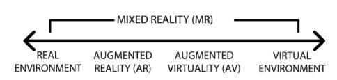
    [5] Milgram P, Kishino F (1994) A taxonomy of mixed reality visual displays. IEICE Transactions on Information and Systems 77: 1321–1329.
    [6] Azuma RT (1997) A survey of augmented reality. Presence: Teleoperators & Virtual Environments 6: 355–385.
    [7] Milgram P, Takemura H, Utsumi A, et al. (1995) Augmented reality: A class of displays on the reality-virtuality continuum. Telemanipulator and Telepresence Technologies 2351: 282–293. International Society for Optics and Photonics. doi: 10.1117/12.197321
    [8] Irizarry J, Gheisari M, Williams G, et al. (2013) InfoSPOT: A mobile Augmented Reality method for accessing building information through a situation awareness approach. Automat Constr 33: 11–23.
    [9] Ibáñez MB, Di Serio Á, Villarán D, et al. (2014) Experimenting with electromagnetism using augmented reality: Impact on flow student experience and educational effectiveness. Comput Educ 71: 1–13. doi: 10.1016/j.compedu.2013.09.004
    [10] Henderson S, Feiner S (2011) Exploring the benefits of augmented reality documentation for maintenance and repair. IEEE transactions on visualization and computer graphics 17: 1355–1368. doi: 10.1109/TVCG.2010.245
    [11] Dow S, Mehta M, Harmon E, et al. (2007) Presence and engagement in an interactive drama. In: Proceedings of the SIGCHI Conference on Human Factors in Computing Systems, pp. 1475–1484, ACM.
    [12] Billinghurst M, Kato H (1999) Collaborative mixed reality. In: Proceedings of the First International Symposium on Mixed Reality, pp. 261–284, Berlin: Springer Verlag.
    [13] Wang X, Dunston PS (2006) Groupware concepts for augmented reality mediated human-to-human collaboration. In: Proceedings of the 23rd Joint International Conference on Computing and Decision Making in Civil and Building Engineering, pp. 1836–1842.
    [14] Brockmann T, Krüger N, Stieglitz S, et al. (2013) A Framework for Collaborative Augmented Reality Applications. In 19th Americas Conference on Information Systems (AMCIS).
    [15] Renevier P, Nigay L (2001) Mobile collaborative augmented reality: the augmented stroll. In: IFIP International Conference on Engineering for Human-Computer Interaction, pp. 299–316, Springer, Berlin, Heidelberg.
    [16] Arias E, Eden H, Fischer G, et al. (2000) Transcending the individual human mind-creating shared understanding through collaborative design. ACM Transactions on Computer-Human Interaction 7: 84–113. doi: 10.1145/344949.345015
    [17] Kim S, Billinghurst M, Lee GA (2018) The Effect of Collaboration Styles and View Independence on Video-Mediated Remote Collaboration. Computer Supported Cooperative Work (CSCW) 27: 569–607.
    [18] Cabral M, Roque G, Nagamura M, et al. (2016) Batmen-Hybrid collaborative object manipulation using mobile devices. In: 2016 IEEE Symposium on3D User Interfaces (3DUI), pp. 275–276.
    [19] Reilly D, Salimian M, MacKay B, et al. (2014) SecSpace: prototyping usable privacy and security for mixed reality collaborative environments. In: Proceedings of the 2014 ACM SIGCHI symposium on Engineering interactive computing systems, pp. 273–282.
    [20] Lin T-H, Liu C-H, Tsai M-H, et al. (2014) Using augmented reality in a multiscreen environment for construction discussion. J Comput Civil Eng 29: 04014088.
    [21] Hollenbeck JR, Ilgen DR, Sego DJ, et al. (1995) Multilevel theory of team decision making: Decision performance in teams incorporating distributed expertise. Journal of Applied Psychology 80: 292–316. doi: 10.1037/0021-9010.80.2.292
    [22] Lightle JP, Kagel JH, Arkes HR (2009) Information exchange in group decision making: The hidden profile problem reconsidered. Manage Sci 55: 568–581. doi: 10.1287/mnsc.1080.0975
    [23] Gül LF, Uzun C, Halıcı SM (2017) Studying Co-design. In: International Conference on Computer-Aided Architectural Design Futures, pp. 212–230.
    [24] Al-Hammad A, Assaf S, Al-Shihah M (1997) The effect of faulty design on building maintenance. Journal of Quality in Maintenance Engineering 3: 29–39. doi: 10.1108/13552519710161526
    [25] Casarin J, Pacqueriaud N, Bechmann D (2018) UMI3D: A Unity3D Toolbox to Support CSCW Systems Properties in Generic 3D User Interfaces. Proceedings of the ACM on Human-Computer Interaction 2: 29.
    [26] Coppens A, Mens T (2018) Towards Collaborative Immersive Environments for Parametric Modelling. In: International Conference on Cooperative Design, Visualization and Engineering, pp. 304–307, Springer.
    [27] Cortés-Dávalos A, Mendoza S (2016) Layout planning for academic exhibits using Augmented Reality. In: 2016 13th International Conference on Electrical Engineering, Computing Science and Automatic Control (CCE), pp. 1–6, IEEE.
    [28] Croft BL, Lucero C, Neurnberger D, et al. (2018) Command and Control Collaboration Sand Table (C2-CST). In: International Conference on Virtual, Augmented and Mixed Reality, pp. 249–259, Springer.
    [29] Dong S, Behzadan AH, Chen F, et al. (2013) Collaborative visualization of engineering processes using tabletop augmented reality. Adv Eng Softw 55: 45–55. doi: 10.1016/j.advengsoft.2012.09.001
    [30] Elvezio C, Ling F, Liu J-S, et al. (2018) Collaborative exploration of urban data in virtual and augmented reality. In: ACM SIGGRAPH 2018 Virtual, Augmented, and Mixed Reality, p. 10, ACM.
    [31] Etzold J, Grimm P, Schweitzer J, et al. (2014) kARbon: a collaborative MR web application for communicationsupport in construction scenarios. In: Proceedings of the companion publication of the 17th ACM conference on Computer supported cooperative work & social computing, pp. 9–12, ACM.
    [32] Flotyński J, Sobociński P (2018) Semantic 4-dimensionai modeling of VR content in a heterogeneous collaborative environment. In: Proceedings of the 23rd International ACM Conference on 3D Web Technology, p. 11, ACM.
    [33] Ibayashi H, Sugiura Y, Sakamoto D, et al. (2015) Dollhouse vr: a multi-view, multi-user collaborative design workspace with vr technology. SIGGRAPH Asia 2015 Emerging Technologies, p. 8, ACM.
    [34] Leon M, Doolan DC, Laing R, et al. (2015) Development of a Computational Design Application for Interactive Surfaces. In: 2015 19th International Conference on Information Visualisation, pp. 506–511, IEEE.
    [35] Li WK, Nee AYC, Ong SK (2018) Mobile augmented reality visualization and collaboration techniques for on-site finite element structural analysis. International Journal of Modeling, Simulation, and Scientific Computing 9: 1840001. doi: 10.1142/S1793962318400019
    [36] Nittala AS, Li N, Cartwright S, et al. (2015) PLANWELL: spatial user interface for collaborative petroleum well-planning. In: SIGGRAPH Asia 2015 Mobile Graphics and Interactive Applications, p. 19, ACM.
    [37] Phan T, Hönig W, Ayanian N (2018) Mixed Reality Collaboration Between Human-Agent Teams. In: 2018 IEEE Conference on Virtual Reality and 3D User Interfaces (VR), pp. 659–660.
    [38] Rajeb SB, Leclercq P (2013) Using spatial augmented reality in synchronous collaborative design. In: International Conference on Cooperative Design, Visualization and Engineering, pp. 1–10, Springer.
    [39] Ro H, Kim I, Byun J, et al. (2018) PAMI: Projection Augmented Meeting Interface for Video Conferencing. In: 2018 ACM Multimedia Conference on Multimedia Conference, pp. 1274–1277, ACM.
    [40] Schattel D, Tönnis M, Klinker G, et al. (2014) On-site augmented collaborative architecture visualization. In: 2014 IEEE International Symposium on Mixed and Augmented Reality (ISMAR), pp. 369–370.
    [41] Shin JG, Ng G, Saakes D (2018) Couples Designing their Living Room Together: a Study with Collaborative Handheld Augmented Reality. In: Proceedings of the 9th Augmented Human International Conference, p. 3, acm.
    [42] Singh AR, Delhi VSK (2018) User behaviour in AR-BIM-based site layout planning. International Journal of Product Lifecycle Management 11: 221–244. doi: 10.1504/IJPLM.2018.094715
    [43] Trout TT, Russell S, Harrison A, et al. (2018) Collaborative mixed reality (MxR) and networked decision making. In: Next-Generation Analyst VI 10653: 106530N. International Society for Optics and Photonics.
    [44] Alhumaidan H, Lo KPY, Selby A (2017) Co-designing with children a collaborative augmented reality book based on a primary school textbook. International Journal of Child-Computer Interaction 15: 24–36.
    [45] Alhumaidan H, Lo KPY, Selby A (2015) Co-design of augmented reality book for collaborative learning experience in primary education. In: 2015 SAI Intelligent Systems Conference (IntelliSys), pp. 427–430, IEEE.
    [46] Benavides X, Amores J, Maes P (2015) Invisibilia: revealing invisible data using augmented reality and internet connected devices. In: Adjunct Proceedings of the 2015 ACM International Joint Conference on Pervasive and Ubiquitous Computing and Proceedings of the 2015 ACM International Symposium on Wearable Computers, pp. 341–344, ACM.
    [47] Blanco-Fernández Y, López-Nores M, Pazos-Arias JJ, et al. (2014) REENACT: A step forward in immersive learning about Human History by augmented reality, role playing and social networking. Expert Syst Appl 41: 4811–4828. doi: 10.1016/j.eswa.2014.02.018
    [48] Boyce MW, Rowan CP, Baity DL, et al. (2017) Using Assessment to Provide Application in Human Factors Engineering to USMA Cadets. In: International Conference on Augmented Cognition, pp. 411–422, Springer.
    [49] Bressler DM, Bodzin AM (2013) A mixed methods assessment of students' flow experiences during a mobile augmented reality science game. Journal of Computer Assisted Learning 29: 505–517. doi: 10.1111/jcal.12008
    [50] Chen M, Fan C, Wu D (2016) Designing Effective Materials and Activities for Mobile Augmented Learning. In: International Conference on Blended Learning, pp. 85–93, Springer.
    [51] Daiber F, Kosmalla F, Krüger A (2013) BouldAR: using augmented reality to support collaborative boulder training. In: CHI' 13 Extended Abstracts on Human Factors in Computing Systems, pp. 949–954, ACM.
    [52] Desai K, Belmonte UHH, Jin R, et al. (2017) Experiences with Multi-Modal Collaborative Virtual Laboratory (MMCVL). In: 2017 IEEE Third International Conference on Multimedia Big Data (BigMM), pp. 376–383, IEEE.
    [53] Fleck S, Simon G (2013) An augmented reality environment for astronomy learning in elementary grades: An exploratory study. In: Proceedings of the 25th Conference on I'Interaction Homme-Machine, p. 14, ACM.
    [54] Gazcón N, Castro S (2015) ARBS: An Interactive and Collaborative System for Augmented Reality Books. In: International Conference on Augmented and Virtual Reality, pp. 89–108, Springer.
    [55] Gelsomini F, Kanev K, Hung P, et al. (2017) BYOD Collaborative Kanji Learning in Tangible Augmented Reality Settings. In: International Conference on Global Research and Education, pp. 315–325, Springer.
    [56] Gironacci IM, Mc-Call R, Tamisier T (2017) Collaborative Storytelling Using Gamification and Augmented Reality. In: International Conference on Cooperative Design, Visualization and Engineering, pp. 90–93, Springer.
    [57] Goyal S, Vijay RS, Monga C, et al. (2016) Code Bits: An Inexpensive Tangible Computational Thinking Toolkit For K-12 Curriculum. In: Proceedings of the TEI'16: Tenth International Conference on Tangible, Embedded, and Embodied Interaction, pp. 441–447, ACM.
    [58] Greenwald SW (2015) Responsive Facilitation of Experiential Learning Through Access to Attentional State. In: Adjunct Proceedings of the 28th Annual ACM Symposium on User Interface Software & Technology, pp. 1–4, ACM.
    [59] Han J, Jo M, Hyun E, et al. (2015) Examining young children's perception toward augmented reality-infused dramatic play. Educational Technology Research and Development 63: 455–474. doi: 10.1007/s11423-015-9374-9
    [60] Iftene A, Trandabăț D (2018) Enhancing the Attractiveness of Learning through Augmented Reality. Procedia Computer Science 126: 166–175. doi: 10.1016/j.procs.2018.07.220
    [61] Jyun-Fong G, Ju-Ling S (2013) The Instructional Application of Augmented Reality in Local History Pervasive Game. pp. 387.
    [62] Kang S, Norooz L, Oguamanam V, et al. (2016) SharedPhys: Live Physiological Sensing, Whole-Body Interaction, and Large-Screen Visualizations to Support Shared Inquiry Experiences. In: Proceedings of the The 15th International Conference on Interaction Design and Children, pp. 275–287, ACM.
    [63] Kazanidis I, Palaigeorgiou G, Papadopoulou Α, et al. (2018) Augmented Interactive Video: Enhancing Video Interactivity for the School Classroom. Journal of Engineering Science and Technology Review 11.
    [64] Keifert D, Lee C, Dahn M, et al. (2017) Agency, Embodiment, & Affect During Play in a Mixed-Reality Learning Environment. In: Proceedings of the 2017 Conference on Interaction Design and Children, pp. 268–277, ACM.
    [65] Kim H-J, Kim B-H (2018) Implementation of young children English education system by AR type based on P2P network service model. Peer-to-Peer Networking and Applications 11: 1252–1264. doi: 10.1007/s12083-017-0612-2
    [66] Krstulovic R, Boticki I, Ogata H (2017) Analyzing heterogeneous learning logs using the iterative convergence method. In: 2017 IEEE 6th International Conference on Teaching, Assessment, and Learning for Engineering, pp. 482–485.
    [67] Le TN, Le YT, Tran MT (2014) Applying Saliency-Based Region of Interest Detection in Developing a Collaborative Active Learning System with Augmented Reality. In: International Conference on Virtual, Augmented and Mixed Reality, pp. 51–62, Springer.
    [68] MacIntyre B, Zhang D, Jones R, et al. (2016) Using projection ar to add design studio pedagogy to a cs classroom. In: 2016 IEEE Virtual Reality (VR), pp. 227–228.
    [69] Malinverni L, Valero C, Schaper MM, et al. (2018) A conceptual framework to compare two paradigms of augmented and mixed reality experiences. In: Proceedings of the 17th ACM Conference on Interaction Design and Children, pp. 7–18, ACM.
    [70] Maskott GK, Maskott MB, Vrysis L (2015) Serious+: A technology assisted learning space based on gaming. In: 2015 International Conference on Interactive Mobile Communication Technologies and Learning (IMCL), pp. 430–432, IEEE.
    [71] Pareto L (2012) Mathematical literacy for everyone using arithmetic games. In: Proceedings of the 9th International Conference on Disability, Virtual Reality and Associated Technologies 9: 87–96. Reading, UK: University of Readings.
    [72] Peters E, Heijligers B, de Kievith J, et al. (2016) Design for collaboration in mixed reality: Technical challenges and solutions. In: 2016 8th International Conference on Games and Virtual Worlds for Serious Applications (VS-GAMES), pp. 1–7, IEEE.
    [73] Punjabi DM, Tung LP, Lin BSP (2013) CrowdSMILE: a crowdsourcing-based social and mobile integrated system for learning by exploration. In: 2013 IEEE 10th International Conference on Ubiquitous Intelligence and Computing and 2013 IEEE 10th International Conference on Autonomic and Trusted Computing, pp. 521–526.
    [74] Rodríguez-Vizzuett L, Pérez-Medina JL, Muñoz-Arteaga J, et al. (2015) Towards the Definition of a Framework for the Management of Interactive Collaborative Learning Applications for Preschoolers. In: Proceedings of the XVI International Conference on Human Computer Interaction, p. 11, ACM.
    [75] Sanabria JC, Arámburo-Lizárraga J (2017) Enhancing 21st Century Skills with AR: Using the Gradual Immersion Method to develop Collaborative Creativity. Eurasia Journal of Mathematics, Science and Technology Education 13: 487–501.
    [76] Shaer O, Valdes C, Liu S, et al. (2014) Designing reality-based interfaces for experiential bio-design. Pers Ubiquit Comput 18: 1515–1532. doi: 10.1007/s00779-013-0752-1
    [77] Shirazi A, Behzadan AH (2015) Content Delivery Using Augmented Reality to Enhance Students' Performance in a Building Design and Assembly Project. Advances in Engineering Education 4.
    [78] Shirazi A, Behzadan AH (2013) Technology-enhanced learning in construction education using mobile context-aware augmented reality visual simulation. In: 2013 Winter Simulations Conference (WSC), pp. 3074–3085, IEEE.
    [79] Sun H, Liu Y, Zhang Z, et al. (2018) Employing Different Viewpoints for Remote Guidance in a Collaborative Augmented Environment. In: Proceedings of the Sixth International Symposium of Chinese CHI, pp. 64–70, ACM.
    [80] Sun H, Zhang Z, Liu Y, et al. (2016) OptoBridge: assisting skill acquisition in the remote experimental collaboration. In: Proceedings of the 28th Australian Conference on Computer-Human Interaction, pp. 195–199, ACM.
    [81] Thompson B, Leavy L, Lambeth A, et al. (2016) Participatory Design of STEM Education AR Experiences for Heterogeneous Student Groups: Exploring Dimensions of Tangibility, Simulation, and Interaction. In: 2016 IEEE International Symposium on Mixed and Augmented Reality (ISMAR-Adjunct), pp. 53–58.
    [82] Wiehr F, Kosmalla F, Daiber F, et al. (2016) betaCube: Enhancing Training for Climbing by a Self-Calibrating Camera-Projection Unit. In: Proceedings of the 2016 CHI Conference Extended Abstracts on Human Factors in Computing Systems, pp. 1998–2004, ACM.
    [83] Yangguang L, Yue L, Xiaodong W (2014) Multiplayer collaborative training system based on Mobile AR innovative interaction technology. In: 2014 International Conference on Virtual Reality and Visualization, pp. 81–85, IEEE.
    [84] Yoon SA, Wang J, Elinich K (2014) Augmented reality and learning in science museums. Digital Systems for Open Access to Formal and Informal Learning, pp. 293–305, Springer.
    [85] Zubir F, Suryani I, Ghazali N (2018) Integration of Augmented Reality into College Yearbook. In: MATEC Web of Conferences 150: 05031. EDP Sciences. doi: 10.1051/matecconf/201815005031
    [86] Dascalu MI, Moldoveanu A, Shudayfat EA (2014) Mixed reality to support new learning paradigms. In: 2014 8th International Conference on System Theory, Control and Computing (ICSTCC), pp. 692–697, IEEE.
    [87] Boonbrahm P, Kaewrat C, Boonbrahm S (2016) Interactive Augmented Reality: A New Approach for Collaborative Learning. In: International Conference on Learning and Collaboration Technologies, pp. 115–124, Springer.
    [88] LaViola Jr JJ, Kruijff E, McMahan RP, et al. (2017) 3D user interfaces: theory and practice. Addison-Wesley Professional.
    [89] Kim S, Lee GA, Sakata N (2013) Comparing pointing and drawing for remote collaboration. In: 2013 IEEE International Symposium on Mixed and Augmented Reality (ISMAR), pp. 1–6, IEEE.
    [90] Akahoshi S, Matsushita M (2018) Magical Projector: Virtual Object Sharing Method among Multiple Users in a Mixed Reality Space. In: 2018 Nicograph International (NicoInt), pp. 70–73, IEEE.
    [91] Baillard C, Fradet M, Alleaume V, et al. (2017) Multi-device mixed reality TV: a collaborative experience with joint use of a tablet and a headset. In: Proceedings of the 23rd ACM Symposium on Virtual Reality Software and Technology, p. 67, ACM.
    [92] Baldauf M, Fröhlich P (2013) The augmented video wall: multi-user AR interaction with public displays. In: CHI'13 Extended Abstracts on Human Factors in Computing Systems, pp. 3015–3018, ACM.
    [93] Ballagas R, Dugan TE, Revelle G, et al. (2013) Electric agents: fostering sibling joint media engagement through interactive television and augmented reality. In: Proceedings of the 2013 conference on Computer supported cooperative work, pp. 225–236, ACM.
    [94] Beimler R, Bruder G, Steinicke F (2013) Smurvebox: A smart multi-user real-time virtual environment for generating character animations. In: Proceedings of the Virtual Reality International Conference: Laval Virtual, p. 1, ACM.
    [95] Bollam P, Gothwal E, Tejaswi V G, et al. (2015) Mobile collaborative augmented reality with real-time AR/VR switching. In: ACM SIGGRAPH 2015 Posters, p. 25, ACM.
    [96] Bourdin P, Sanahuja JMT, Moya CC, et al. (2013) Persuading people in a remote destination to sing by beaming there. In: Proceedings of the 19th ACM Symposium on Virtual Reality Software and Technology, pp. 123–132, ACM.
    [97] Brondi R, Avveduto G, Alem L, et al. (2015) Evaluating the effects of competition vs collaboration on user engagement in an immersive game using natural interaction. In: Proceedings of the 21st ACM Symposium on Virtual Reality Software and Technology, p. 191, ACM.
    [98] Ch'ng E, Harrison D, Moore S (2017) Shift-life interactive art: Mixed-reality artificial ecosystem simulation. Presence: Teleoperators & Virtual Environments 26: 157–181.
    [99] Courchesne L, Durand E, Roy B (2014) Posture platform and the drawing room: virtual teleportation in cyberspace. Leonardo 47: 367–374. doi: 10.1162/LEON_a_00842
    [100] Dal Corso A, Olsen M, Steenstrup KH, et al. (2015) VirtualTable: a projection augmented reality game. In: SIGGRAPH Asia 2015 Posters, p. 40, ACM.
    [101] Datcu D, Lukosch S, Lukosch H (2016) A Collaborative Game to Study Presence and Situational Awareness in a Physical and an Augmented Reality Environment. J Univers Comput Sci 22: 247–270.
    [102] Datcu D, Lukosch SG, Lukosch HK (2014) A collaborative game to study the perception of presence during virtual co-location. In: Proceedings of the companion publication of the 17th ACM conference on Computer supported cooperative work & social computing, pp. 5–8, ACM.
    [103] Figueroa P, Hernández JT, Merienne F, et al. (2018) Heterogeneous, distributed mixed reality Applications. A concept. In: 2018 IEEE Conference on Virtual Reality and 3D User Interfaces (VR), pp. 549–550.
    [104] Fischbach M, Lugrin J-L, Brandt M, et al. (2018) Follow the White Robot-A Role-Playing Game with a Robot Game Master. In: Proceedings of the 17th International Conference on Autonomous Agents and MultiAgent Systems, pp. 1812–1814.
    [105] Fischbach M, Striepe H, Latoschik ME, et al. (2016) A low-cost, variable, interactive surface for mixed-reality tabletop games. In: Proceedings of the 22nd ACM Conference on Virtual Reality Software and Technology, pp. 297–298, ACM.
    [106] Günther S, Müller F, Schmitz M, et al. (2018) CheckMate: Exploring a Tangible Augmented Reality Interface for Remote Interaction. In: Extended Abstracts of the 2018 CHI Conference on Human Factors in Computing Systems, p. LBW570, ACM.
    [107] Huo K, Wang T, Paredes L, et al. (2018) SynchronizAR: Instant Synchronization for Spontaneous and Spatial Collaborations in Augmented Reality. In: Proceedings of the 31st Annual ACM Symposium on User Interface Software and Technology, pp. 19–30, ACM.
    [108] Karakottas A, Papachristou A, Doumanoqlou A, et al. (2018) Augmented VR. In: 2018 IEEE Conference on Virtual Reality and 3D User Interfaces (VR), pp. 18–22, IEEE.
    [109] Lantin M, Overstall SL, Zhao H (2018) I am afraid: voice as sonic sculpture. In: ACM SIGGRAPH 2018 Posters, pp. 1–2, ACM.
    [110] Loviska M, Krause O, Engelbrecht HA, et al. (2016) Immersed gaming in Minecraft. In: Proceedings of the 7th International Conference on Multimedia Systems, p. 32, ACM.
    [111] Mackamul EB, Esteves A (2018) A Look at the Effects of Handheld and Projected Augmented-reality on a Collaborative Task. In: Proceedings of the Symposium on Spatial User Interaction, pp. 74–78, ACM.
    [112] Margolis T, Cornish T (2013) Vroom: designing an augmented environment for remote collaboration in digital cinema production. In: The Engineering Reality of Virtual Reality 2013 8649: 86490F. International Society for Optics and Photonics. doi: 10.1117/12.2008587
    [113] McGill M, Williamson JH, Brewster SA (2016) Examining the role of smart TVs and VR HMDs in synchronous at-a-distance media consumption. ACM T Comput-Hum Int 23: 33.
    [114] Mechtley B, Stein J, Roberts C, et al. (2017) Rich State Transitions in a Media Choreography Framework Using an Idealized Model of Cloud Dynamics. In: Proceedings of the onThematic Workshops of ACM Multimedia 2017, pp. 477–484, ACM.
    [115] Pillias C, Robert-Bouchard R, Levieux G (2014) Designing tangible video games: lessons learned from the sifteo cubes. In: Proceedings of the SIGCHI Conference on Human Factors in Computing Systems, pp. 3163–3166, ACM.
    [116] Podkosova I, Kaufmann H (2018) Co-presence and proxemics in shared walkable virtual environments with mixed collocation. In: Proceedings of the 24th ACM Symposium on Virtual Reality Software and Technology, pp. 21, ACM.
    [117] Prins MJ, Gunkel SN, Stokking HM, et al. (2018) TogetherVR: A framework for photorealistic shared media experiences in 360-degree VR. SMPTE Motion Imag J 127: 39–44.
    [118] Rostami A, Bexell E, Stanisic S (2018) The Shared Individual. In: Proceedings of the Twelfth International Conference on Tangible, Embedded, and Embodied Interaction, pp. 511–516, ACM.
    [119] Sato T, Hwang DH, Koike H (2018) MlioLight: Projector-camera Based Multi-layered Image Overlay System for Multiple Flashlights Interaction. In: Proceedings of the 2018 ACM International Conference on Interactive Surfaces and Spaces, pp. 263–271, ACM.
    [120] Spielmann S, Schuster A, Götz K, et al. (2016) VPET: a toolset for collaborative virtual filmmaking. In: SIGGRAPH ASIA 2016 Technical Briefs, p. 29, ACM.
    [121] Trottnow J, Götz K, Seibert S, et al. (2015) Intuitive virtual production tools for set and light editing. In: Proceedings of the 12th European Conference on Visual Media Production, p. 6, ACM.
    [122] Valverde I, Cochrane T (2017) Senses Places: soma-tech mixed-reality participatory performance installation/environment. In: Proceedings of the 8th International Conference on Digital Arts, pp. 195–197, ACM.
    [123] Van Troyer A (2013) Enhancing site-specific theatre experience with remote partners in sleep no more. In: Proceedings of the 2013 ACM International workshop on Immersive media experiences, pp. 17–20, ACM.
    [124] Vermeer J, Alaka S, de Bruin N, et al. (2018) League of lasers: a superhuman sport using motion tracking. In: Proceedings of the First Superhuman Sports Design Challenge on First International Symposium on Amplifying Capabilities and Competing in Mixed Realities, p. 8, ACM.
    [125] Wegner K, Seele S, Buhler H, et al. (2017) Comparison of Two Inventory Design Concepts in a Collaborative Virtual Reality Serious Game. In: Extended Abstracts Publication of the Annual Symposium on Computer-Human Interaction in Play, pp. 323–329, ACM.
    [126] Zhou Q, Hagemann G, Fels S, et al. (2018) Coglobe: a co-located multi-person FTVR experience. In: ACM SIGGRAPH 2018 Emerging Technologies, p. 5, ACM.
    [127] Zimmerer C, Fischbach M, Latoschik ME (2014) Fusion of Mixed-Reality Tabletop and Location-Based Applications for Pervasive Games. In: Proceedings of the Ninth ACM International Conference on Interactive Tabletops and Surfaces, pp. 427–430, ACM.
    [128] Speicher M, Hall BD, Yu A, et al. (2018) XD-AR: Challenges and Opportunities in Cross-Device Augmented Reality Application Development. Proceedings of the ACM on Human-Computer Interaction 2: 7.
    [129] Gauglitz S, Nuernberger B, Turk M, et al. (2014) World-stabilized annotations and virtual scene navigation for remote collaboration. In: Proceedings of the 27th Annual ACM symposium on User interface software and technology, pp. 449–459, ACM.
    [130] Abramovici M, Wolf M, Adwernat S, et al. (2017) Context-aware Maintenance Support for Augmented Reality Assistance and Synchronous Multi-user Collaboration. Procedia CIRP 59: 18–22. doi: 10.1016/j.procir.2016.09.042
    [131] Aschenbrenner D, Li M, Dukalski R, et al. (2018) Collaborative Production Line Planning with Augmented Fabrication. In: 2018 IEEE Conference on Virtual Reality and 3D User Interfaces (VR), pp. 509–510, IEEE.
    [132] Bednarz T, James C, Widzyk-Capehart E, et al. (2015) Distributed collaborative immersive virtual reality framework for the mining industry. Machine Vision and Mechatronics in Practice, pp. 39–48, Springer.
    [133] Capodieci A, Mainetti L, Alem L (2015) An innovative approach to digital engineering services delivery: An application in maintenance. In: 2015 11th International Conference on Innovations in Information Technology (IIT), pp. 342–349, IEEE.
    [134] Choi SH, Kim M, Lee JY (2018) Situation-dependent remote AR collaborations: Image-based collaboration using a 3D perspective map and live video-based collaboration with a synchronized VR mode. Comput Ind 101: 51–66. doi: 10.1016/j.compind.2018.06.006
    [135] Clergeaud D, Roo JS, Hachet M, et al. (2017) Towards seamless interaction between physical and virtual locations for asymmetric collaboration. In: Proceedings of the 23rd ACM Symposium on Virtual Reality Software and Technology, pp. 1–4, ACM.
    [136] Datcu D, Cidota M, Lukosch SG, et al. (2014) Virtual co-location to support remote assistance for inflight maintenance in ground training for space missions. In: Proceedings of the 15th International Conference on Computer Systems and Technologies, pp. 134–141, ACM.
    [137] Domova V, Vartiainen E, Englund M (2014) Designing a remote video collaboration system for industrial settings. In: Proceedings of the Ninth ACM International Conference on Interactive Tabletops and Surfaces, pp. 229–238, ACM.
    [138] Elvezio C, Sukan M, Oda O, et al. (2017) Remote collaboration in AR and VR using virtual replicas. In: ACM SIGGRAPH 2017 VR Village, p. 13, ACM.
    [139] Funk M, Kritzler M, Michahelles F (2017) HoloCollab: A Shared Virtual Platform for Physical Assembly Training using Spatially-Aware Head-Mounted Displays. In: Proceedings of the Seventh International Conference on the Internet of Things, p. 19, ACM.
    [140] Galambos P, Csapó ÁB, Zentay PZ, et al. (2015) Design, programming and orchestration of heterogeneous manufacturing systems through VR-powered remote collaboration. Robotics and Computer-Integrated Manufacturing 33: 68–77. doi: 10.1016/j.rcim.2014.08.012
    [141] Galambos P, Baranyi PZ, Rudas IJ (2014) Merged physical and virtual reality in collaborative virtual workspaces: The VirCA approach. In: IECON 2014 – 40th Annual Conference of the IEEE Industrial Electronics Society, pp. 2585–2590, IEEE.
    [142] Gupta RK, Ucler C, Bernard A (2018) Extension of the Virtual Customer Inspection for Distant Collaboration in NPD. In: 2018 IEEE International Conference on Engineering, Technology and Innovation, pp. 1–7.
    [143] Gurevich P, Lanir J, Cohen B (2015) Design and implementation of teleadvisor: a projection-based augmented reality system for remote collaboration. Computer Supported Cooperative Work (CSCW) 24: 527–562. doi: 10.1007/s10606-015-9232-7
    [144] Günther S, Kratz SG, Avrahami D, et al. (2018) Exploring Audio, Visual, and Tactile Cues for Synchronous Remote Assistance. In: Proceedings of the 11th Pervasive Technologies Related to Assistive Environments Conference, pp. 339–344, ACM.
    [145] Morosi F, Carli I, Caruso G, et al. (2018) Analysis of Co-Design Scenarios and Activities for the Development of A Spatial-Augmented Reality Design Platform. In: DS 92: Proceedings of the DESIGN 2018 15th International Design Conference, pp. 381–392.
    [146] Plopski A, Fuvattanasilp V, Poldi J, et al. (2018) Efficient In-Situ Creation of Augmented Reality Tutorials. In: 2018 Workshop on Metrology for Industry 4.0 and IoT, pp. 7–11, IEEE.
    [147] Seo D-W, Lee S-M, Park K-S, et al. (2015) INTEGRATED ENGINEERING PRODUCT DESIGN SIMULATION PLATFORM FOR COLLABORATIVE SIMULATION UNDER THE USER EXPERIENCE OF SME USERS. simulation 1: 2.
    [148] Zenati N, Hamidia M, Bellarbi A, et al. (2015) E-maintenance for photovoltaic power system in Algeria. In: 2015 IEEE International Conference on Industrial Technology, pp. 2594–2599.
    [149] Zenati N, Benbelkacem S, Belhocine M, et al. (2013) A new AR interaction for collaborative E-maintenance system. IFAC Proceedings Volumes 46: 619–624.
    [150] Zenati-Henda N, Bellarbi A, Benbelkacem S, et al. (2014) Augmented reality system based on hand gestures for remote maintenance. In: 2014 International Conference on Multimedia Computing and Systems (ICMCS), pp. 5–8, IEEE.
    [151] Huang W, Billinghurst M, Alem L, et al. (2018) HandsInTouch: sharing gestures in remote collaboration. In: Proceedings of the 30th Australian Conference on Computer-Human Interaction, pp. 396–400, ACM.
    [152] Davis MC, Can DD, Pindrik J, et al. (2016) Virtual interactive presence in global surgical education: international collaboration through augmented reality. World neurosurgery 86: 103–111. doi: 10.1016/j.wneu.2015.08.053
    [153] Alharthi SA, Sharma HN, Sunka S, et al. (2018) Designing Future Disaster Response Team Wearables from a Grounding in Practice. In: Proceedings of the Technology, Mind, and Society, p. 1, ACM.
    [154] Carbone M, Freschi C, Mascioli S, et al. (2016) A wearable augmented reality platform for telemedicine. In: International Conference on Augmented Reality, Virtual Reality and Computer Graphics, pp. 92–100, Springer.
    [155] Elvezio C, Ling F, Liu J-S, et al. (2018) Collaborative Virtual Reality for Low-Latency Interaction. In: The 31st Annual ACM Symposium on User Interface Software and Technology Adjunct Proceedings, pp. 179–181, ACM.
    [156] Gillis J, Calyam P, Apperson O, et al. (2016) Panacea's Cloud: Augmented reality for mass casualty disaster incident triage and co-ordination. In: 2016 13th IEEE Annual Consumer Communications & Networking Conference (CCNC), pp. 264–265, IEEE.
    [157] Kurillo G, Yang AY, Shia V, et al. (2016) New emergency medicine paradigm via augmented telemedicine. In: 8th International Conference on Virtual, Augmented and Mixed Reality, VAMR 2016 and Held as Part of 18th International Conference on Human-Computer Interaction, HCI International 2016, pp. 502–511, Springer.
    [158] Nunes M, Nedel LP, Roesler V (2013) Motivating people to perform better in exergames: Collaboration vs. competition in virtual environments. In: 2013 IEEE Virtual Reality (VR), pp. 115–116, IEEE.
    [159] Nunes IL, Lucas R, Simões-Marques M, et al. (2017) Augmented Reality in Support of Disaster Response. In: International Conference on Applied Human Factors and Ergonomics, pp. 155–167, Springer.
    [160] Popescu D, Lăptoiu D, Marinescu R, et al. (2017) Advanced Engineering in Orthopedic Surgery Applications. Key Engineering Materials 752: 99–104. doi: 10.4028/www.scientific.net/KEM.752.99
    [161] Shluzas LA, Aldaz G, Leifer L (2016) Design Thinking Health: Telepresence for Remote Teams with Mobile Augmented Reality. In: Design Thinking Research, pp. 53–66, Springer.
    [162] Sirilak S, Muneesawang P (2018) A New Procedure for Advancing Telemedicine Using the HoloLens. IEEE Access 6: 60224–60233. doi: 10.1109/ACCESS.2018.2875558
    [163] Vassell M, Apperson O, Calyam P, et al. (2016) Intelligent Dashboard for augmented reality based incident command response co-ordination. In: 2016 13th IEEE Annual Consumer Communications & Networking Conference (CCNC), pp. 976–979, IEEE.
    [164] Bach B, Sicat R, Beyer J, et al. (2018) The Hologram in My Hand: How Effective is Interactive Exploration of 3D Visualizations in Immersive Tangible Augmented Reality? IEEE Transactions on Visualization & Computer Graphics 24: 457–467.
    [165] Daher S (2017) Optical see-through vs. spatial augmented reality simulators for medical applications. In: 2017 IEEE Virtual Reality (VR), pp. 417–418.
    [166] Camps-Ortueta I, Rodríguez-Muñoz JM, Gómez-Martín PP, et al. (2017) Combining augmented reality with real maps to promote social interaction in treasure hunts. CoSECivi, pp. 131–143.
    [167] Chen H, Lee AS, Swift M, et al. (2015) 3D collaboration method over HoloLens™ and Skype™ end points. In: Proceedings of the 3rd International Workshop on Immersive Media Experiences, pp. 27–30, ACM.
    [168] Gleason C, Fiannaca AJ, Kneisel M, et al. (2018) FootNotes: Geo-referenced Audio Annotations for Nonvisual Exploration. Proceedings of the ACM on Interactive, Mobile, Wearable and Ubiquitous Technologies 2: 109.
    [169] Huang W, Kaminski B, Luo J, et al. (2015) SMART: design and evaluation of a collaborative museum visiting application. In: 12th International Conference, CDVE 2015 – Cooperative Design, Visualization, and Engineering 12th International Conference 9320: 57–64.
    [170] Kallioniemi P, Heimonen T, Turunen M, et al. (2015) Collaborative navigation in virtual worlds: how gender and game experience influence user behavior. In: Proceedings of the 21st ACM Symposium on Virtual Reality Software and Technology, pp. 173–182, ACM.
    [171] Li N, Nittala AS, Sharlin E, et al. (2014) Shvil: collaborative augmented reality land navigation. In: CHI'14 Extended Abstracts on Human Factors in Computing Systems, pp. 1291–1296, ACM.
    [172] Nuernberger B, Lien K-C, Grinta L, et al. (2016) Multi-view gesture annotations in image-based 3D reconstructed scenes. In: Proceedings of the 22nd ACM Conference on Virtual Reality Software and Technology, pp. 129–138, ACM.
    [173] Kallioniemi P, Hakulinen J, Keskinen T, et al. (2013) Evaluating landmark attraction model in collaborative wayfinding in virtual learning environments. In: Proceedings of the 12th International Conference on Mobile and Ubiquitous Multimedia, pp. 1–10, ACM.
    [174] Bork F, Schnelzer C, Eck U, et al. (2018) Towards Efficient Visual Guidance in Limited Field-of-View Head-Mounted Displays. IEEE transactions on visualization and computer graphics 24: 2983–2992. doi: 10.1109/TVCG.2018.2868584
    [175] Sodhi RS, Jones BR, Forsyth D, et al. (2013) BeThere: 3D mobile collaboration with spatial input. In: Proceedings of the SIGCHI Conference on Human Factors in Computing Systems, pp. 179–188, ACM.
    [176] Lien K-C, Nuernberger B, Turk M, et al. (2015) [POSTER] 2D-3D Co-segmentation for AR-based Remote Collaboration. In: 2015 IEEE International Symposium on Mixed and Augmented Reality, pp. 184–185, IEEE.
    [177] Nuernberger B, Lien K-C, Höllerer T, et al. (2016) Anchoring 2D gesture annotations in augmented reality. In: 2016 IEEE Virtual Reality (VR), pp. 247–248, IEEE.
    [178] Nuernberger B, Lien K-C, Höllerer T, et al. (2016) Interpreting 2d gesture annotations in 3d augmented reality. In: 2016 IEEE Symposium on 3D User Interfaces (3DUI), pp. 149–158.
    [179] Kovachev D, Nicolaescu P, Klamma R (2014) Mobile real-time collaboration for semantic multimedia. Mobile Networks and Applications 19: 635–648. doi: 10.1007/s11036-013-0453-z
    [180] You S, Thompson CK (2017) Mobile collaborative mixed reality for supporting scientific inquiry and visualization of earth science data. In: 2017 IEEE Virtual Reality (VR), pp. 241–242.
    [181] Wiehr F, Daiber F, Kosmalla F, et al. (2017) ARTopos: augmented reality terrain map visualization for collaborative route planning. In: Proceedings of the 2017 ACM International Joint Conference on Pervasive and Ubiquitous Computing and Proceedings of the 2017 ACM International Symposium on Wearable Computers, pp. 1047–1050, ACM.
    [182] Müller J, Rädle R, Reiterer H (2017) Remote Collaboration With Mixed Reality Displays: How Shared Virtual Landmarks Facilitate Spatial Referencing. In: Proceedings of the 2017 CHI Conference on Human Factors in Computing Systems, pp. 6481–6486, ACM.
    [183] Park S, Kim J (2018) Augmented Memory: Site-Specific Social Media with AR. In: Proceedings of the 9th Augmented Human International Conference, p. 41, ACM.
    [184] Ryskeldiev B, Igarashi T, Zhang J, et al. (2018) Spotility: Crowdsourced Telepresence for Social and Collaborative Experiences in Mobile Mixed Reality. In: Companion of the 2018 ACM Conference on Computer Supported Cooperative Work and Social Computing, pp. 373–376, ACM.
    [185] Grandi JG, Berndt I, Debarba HG, et al. (2017) Collaborative manipulation of 3D virtual objects in augmented reality scenarios using mobile devices. In: 2017 IEEE Symposium on 3D User Interfaces (3DUI), pp. 264–265, IEEE.
    [186] Cortés-Dávalos A, Mendoza S (2016) AR-based Modeling of 3D Objects in Multi-user Mobile Environments. In: CYTED-RITOS International Workshop on Groupware, pp. 21–36, Springer.
    [187] Cortés-Dávalos A, Mendoza S (2016) Augmented Reality-Based Groupware for Editing 3D Surfaces on Mobile Devices. In: 2016 International Conference on Collaboration Technologies and Systems (CTS), pp. 319–326, IEEE.
    [188] Zhang W, Han B, Hui P, et al. (2018) CARS: Collaborative Augmented Reality for Socialization. In: Proceedings of the 19th International Workshop on Mobile computing Systems & Applications, pp. 25–30, ACM.
    [189] Cortés-Dávalos A, Mendoza S (2016) Collaborative Web Authoring of 3D Surfaces Using Augmented Reality on Mobile Devices. In: 2016 IEEE/WIC/ACM International Conference on Web Intelligence (WI), pp. 640–643, IEEE.
    [190] Pani M, Poiesi F (2018) Distributed Data Exchange with Leap Motion. International Conference on Augmented Reality, Virtual Reality, and Computer Graphics, pp. 655–667, Springer.
    [191] Grandi JG, Debarba HG, Bemdt I, et al. (2018) Design and Assessment of a Collaborative 3D Interaction Technique for Handheld Augmented Reality. In: 2018 IEEE Conference on Virtual Reality and 3D User Interfaces (VR), pp. 49–56.
    [192] Müller J, Rädle R, Reiterer H (2016) Virtual Objects as Spatial Cues in Collaborative Mixed Reality Environments: How They Shape Communication Behavior and User Task Load. In: Proceedings of the 2016 CHI Conference on Human Factors in Computing Systems, pp. 1245–1249, ACM.
    [193] Müller J, Butscher S, Feyer SP, et al. (2017) Studying collaborative object positioning in distributed augmented realities. In: Proceedings of the 16th International Conference on Mobile and Ubiquitous Multimedia, pp. 123–132, ACM.
    [194] Francese R, Passero I, Zarraonandia T (2012) An augmented reality application to gather participant feedback during a meeting. In: Information systems: crossroads for organization, management, accounting and engineering, pp. 173–180.
    [195] Datcu D, Lukosch SG, Lukosch HK (2016) Handheld Augmented Reality for Distributed Collaborative Crime Scene Investigation. In: Proceedings of the 19th International Conference on Supporting Group Work, pp. 267–276, ACM.
    [196] Pece F, Steptoe W, Wanner F, et al. (2013) Panoinserts: mobile spatial teleconferencing. In: Proceedings of the SIGCHI Conference on Human Factors in Computing Systems, pp. 1319–1328, ACM.
    [197] Cai M, Masuko S, Tanaka J (2018) Gesture-based Mobile Communication System Providing Side-by-side Shopping Feeling. In: Proceedings of the 23rd International Conference on Intelligent User Interfaces Companion, p. 2, ACM.
    [198] Chang YS, Nuernberger B, Luan B, et al. (2017) Gesture-based augmented reality annotation. In: 2017 IEEE Virtual Reality (VR), pp. 469–470, IEEE.
    [199] Le Chénéchal M, Duval T, Gouranton V, et al. (2016) Vishnu: virtual immersive support for helping users an interaction paradigm for collaborative remote guiding in mixed reality. In: 2016 IEEE Third VR International Workshop on Collaborative virtual Environments (3DCVE), pp. 9–12.
    [200] Piumsomboon T, Lee Y, Lee GA, et al. (2017) Empathic Mixed Reality: Sharing What You Feel and Interacting with What You See. In: 2017 International Symposium on Ubiquitous Virtual Reality (ISUVR), pp. 38–41, IEEE.
    [201] Piumsomboon T, Lee Y, Lee G, et al. (2017) CoVAR: a collaborative virtual and augmented reality system for remote collaboration. In: SIGGRAPH Asia 2017 Emerging Technologies, p. 3, ACM.
    [202] Lee Y, Masai K, Kunze KS, et al. (2016) A Remote Collaboration System with Empathy Glasses. In: 2016 IEEE International Symposium on Mixed and Augmented Reality (ISMAR-Adjunct), pp. 342–343, IEEE.
    [203] Piumsomboon T, Dey A, Ens B, et al. (2017) [POSTER] CoVAR: Mixed-Platform Remote Collaborative Augmented and Virtual Realities System with Shared Collaboration Cues. In: 2017 IEEE International Symposium on Mixed and Augmented Reality (ISMAR-Adjunct), pp. 218–219, IEEE.
    [204] Piumsomboon T, Day A, Ens B, et al. (2017) Exploring enhancements for remote mixed reality collaboration. In: SIGGRAPH Asia 2017 Mobile Graphics & Interactive Applications, p. 16, ACM.
    [205] Amores J, Benavides X, Maes P (2015) Showme: A remote collaboration system that supports immersive gestural communication. In: Proceedings of the 33rd Annual ACM Conference Extended Abstracts on Human Factors in Computing Systems, pp. 1343–1348, ACM.
    [206] Yu J, Noh S, Jang Y, et al. (2015) A hand-based collaboration framework in egocentric coexistence reality. In: 2015 12th International Conference on Ubiquitous Robots and Ambient Intelligence (URAI), pp. 545–548, IEEE.
    [207] Piumsomboon T, Lee GA, Hart JD, et al. (2018) Mini-Me: An Adaptive Avatar for Mixed Reality Remote Collaboration. In: Proceedings of the 2018 CHI Conference on Human Factors in Computing Systems, p. 46, ACM.
    [208] Piumsomboon T, Lee GA, Billinghurst M (2018) Snow Dome: A Multi-Scale Interaction in Mixed Reality Remote Collaboration. In: Extended Abstracts of the 2018 CHI Conference on Human Factors in Computing Systems, p. D115, ACM.
    [209] Cidota M, Lukosch S, Datcu D, et al. (2016) Workspace awareness in collaborative AR using HMDS: a user study comparing audio and visual notifications. In: Proceedings of the 7th Augmented Human International Conference 2016, p. 3, ACM.
    [210] Jo D, Kim K-H, Kim GJ (2016) Effects of avatar and background representation forms to co-presence in mixed reality (MR) tele-conference systems. In: SIGGRAPH Asia 2016 Virtual Reality meets Physical Reality: Modelling and Simulating Virtual Humans and Environments, p. 12, ACM.
    [211] Yu J, Jeon J-u, Park G, et al. (2016) A Unified Framework for Remote Collaboration Using Interactive AR Authoring and Hands Tracking. In: International Conference on Distributed, Ambient, and Pervasive Interactions, pp. 132–141, Springer.
    [212] Nassani A, Lee G, Billinghurst M, et al. (2017) [POSTER] The Social AR Continuum: Concept and User Study. In: 2017 IEEE International Symposium on Mixed and Augmented Reality (ISMAR-Adjunct), pp. 7–8.
    [213] Gao L, Bai H, Lee G, et al. (2016) An oriented point-cloud view for MR remote collaboration. SIGGRAPH ASIA 2016 Mobile Graphics and Interactive Applications, p. 8, ACM.
    [214] Lee GA, Teo T, Kim S, et al. (2017) Mixed reality collaboration through sharing a live panorama. SIGGRAPH Asia 2017 Mobile Graphics & Interactive Applications, p. 14, ACM.
    [215] Gao L, Bai H, Lindeman R, et al. (2017) Static local environment capturing and sharing for MR remote collaboration. SIGGRAPH Asia 2017 Mobile Graphics & Interactive Applications, p. 17, ACM.
    [216] Lee GA, Teo T, Kim S, et al. (2017) Sharedsphere: MR collaboration through shared live panorama. SIGGRAPH Asia 2017 Emerging Technologies, pp. 1–2, ACM.
    [217] Rühmann LM, Prilla M, Brown G (2018) Cooperative Mixed Reality: An Analysis Tool. In: Proceedings of the 2018 ACM Conference on Supporting Groupwork, pp. 107–111, ACM.
    [218] Lee H, Ha T, Noh S, et al. (2013) Context-of-Interest Driven Trans-Space Convergence for Spatial Co-presence. In: Proceedings of the First International Conference on Distributed, Ambient, and Pervasive Interactions 8028: 388–395. doi: 10.1007/978-3-642-39351-8_42
    [219] Yang P, Kitahara I, Ohta Y. (2015) [POSTER] Remote Mixed Reality System Supporting Interactions with Virtualized Objects. In: 2015 IEEE International Symposium on Mixed and Augmented Reality, pp. 64–67, IEEE.
    [220] Benbelkacem S, Zenati-Henda N, Belghit H, et al. (2015) Extended web services for remote collaborative manipulation in distributed augmented reality. In: 2015 3rd International Conference on Control, Engineering & Information Technology (CEIT), pp. 1–5, IEEE.
    [221] Pan Y, Sinclair D, Mitchell K (2018) Empowerment and embodiment for collaborative mixed reality systems. Comput Animat Virt W 29: e1838. doi: 10.1002/cav.1838
    [222] Drochtert D, Geiger C (2015) Collaborative magic lens graph exploration. In: SIGGRAPH Asia 2015 Mobile Graphics and Interactive Applications, p. 25, ACM.
    [223] Lee J-Y, Kwon J-H, Nam S-H, et al. (2016) Coexistent Space: Collaborative Interaction in Shared 3D Space. In: Proceedings of the 2016 Symposium on Spatial User Interaction, pp. 175–175, ACM.
    [224] Müller F, Günther S, Nejad AH, et al. (2017) Cloudbits: supporting conversations through augmented zero-query search visualization. In: Proceedings of the 5th Symposium on Spatial User Interaction, pp. 30–38, ACM.
    [225] Lehment NH, Tiefenbacher P, Rigoll G (2014) Don't Walk into Walls: Creating and Visualizing Consensus Realities for Next Generation Videoconferencing. In: Proceedings, Part I, of the 6th International Conference on Virtual, Augmented and Mixed Reality. Designing and Developing Virtual and Augmented Environments 8525: 170–180.
    [226] Roth D, Lugrin J-L, Galakhov D, et al. (2016) Avatar realism and social interaction quality in virtual reality. In: 2016 IEEE Virtual Reality (VR), pp. 277–278, IEEE.
    [227] Kasahara S, Nagai S, Rekimoto J (2017) JackIn Head: Immersive visual telepresence system with omnidirectional wearable camera. IEEE transactions on visualization and computer graphics 23: 1222–1234. doi: 10.1109/TVCG.2016.2642947
    [228] Luongo C, Leoncini P (2018) An UE4 Plugin to Develop CVE Applications Leveraging Participant's Full Body Tracking Data. International Conference on Augmented Reality, Virtual Reality, and Computer Graphics, pp. 610–622.
    [229] Piumsomboon T, Lee GA, Ens B, et al. (2018) Superman vs Giant: A Study on Spatial Perception for a Multi-Scale Mixed Reality Flying Telepresence Interface. IEEE Transactions on Visualization and Computer Graphics 24: 2974–2982. doi: 10.1109/TVCG.2018.2868594
    [230] Kasahara S, Rekimoto J (2015) JackIn head: immersive visual telepresence system with omnidirectional wearable camera for remote collaboration. In: Proceedings of the 21st ACM Symposium on Virtual Reality Software and Technology, pp. 217–225, ACM.
    [231] Adams H, Thompson C, Thomas D, et al. (2015) The effect of interpersonal familiarity on cooperation in a virtual environment. In: Proceedings of the ACM SIGGRAPH Symposium on Applied Perception, pp. 138–138, ACM.
    [232] Ryskeldiev B, Cohen M, Herder J (2017) Applying rotational tracking and photospherical imagery to immersive mobile telepresence and live video streaming groupware. In: SIGGRAPH Asia 2017 Mobile Graphics & Interactive Applications, p. 5.
    [233] Mai C, Bartsch SA, Rieger L (2018) Evaluating Shared Surfaces for Co-Located Mixed-Presence Collaboration. In: Proceedings of the 17th International Conference on Mobile and Ubiquitous Multimedia, pp. 1–5, ACM.
    [234] Congdon BJ, Wang T, Steed A (2018) Merging environments for shared spaces in mixed reality. In: Proceedings of the 24th ACM Symposium on Virtual Reality Software and Technology, p. 11.
    [235] Gao L, Bai H, He W, et al. (2018) Real-time visual representations for mobile mixed reality remote collaboration. SIGGRAPH Asia 2018 Virtual & Augmented Reality, p. 15.
    [236] Lee G, Kim S, Lee Y, et al. (2017) [POSTER] Mutually Shared Gaze in Augmented Video Conference. In: 2017 IEEE International Symposium on Mixed and Augmented Reality (ISMAR-Adjunct), pp. 79–80, IEEE.
    [237] Tiefenbacher P, Gehrlich T, Rigoll G (2015) Impact of annotation dimensionality under variable task complexity in remote guidance. In: 2015 IEEE Symposium on 3D User Interfaces (3DUI), pp. 189–190, IEEE.
    [238] Adcock M, Gunn C (2015) Using Projected Light for Mobile Remote Guidance. Computer Supported Cooperative Work (CSCW) 24: 591–611. doi: 10.1007/s10606-015-9237-2
    [239] Kim S, Lee GA, Ha S, et al. (2015) Automatically freezing live video for annotation during remote collaboration. In: Proceedings of the 33rd Annual ACM Conference Extended Abstracts on Human Factors in Computing Systems, pp. 1669–1674, ACM.
    [240] Tait M, Billinghurst M (2015) The effect of view independence in a collaborative AR system. Computer Supported Cooperative Work (CSCW) 24: 563–589. doi: 10.1007/s10606-015-9231-8
    [241] Adcock M, Anderson S, Thomas B (2013) RemoteFusion: real time depth camera fusion for remote collaboration on physical tasks. In: Proceedings of the 12th ACM SIGGRAPH International Conference on Virtual-Reality Continuum and Its Applications in Industry, pp. 235–242, ACM.
    [242] Kim S, Lee GA, Sakata N, et al. (2013) Study of augmented gesture communication cues and view sharing in remote collaboration. In: 2013 IEEE International Symposium on Mixed and Augmented Reality, pp. 261–262, IEEE.
    [243] Sakata N, Takano Y, Nishida S (2014) Remote Collaboration with Spatial AR Support. In: International Conference on Human-Computer Interaction, pp. 148–157, Springer.
    [244] Tiefenbacher P, Gehrlich T, Rigoll G, et al. (2014) Supporting remote guidance through 3D annotations. In: Proceedings of the 2nd ACM Symposium on Spatial User Interaction, pp. 141–141, ACM.
    [245] Tait M, Billinghurst M (2014) View independence in remote collaboration using AR. ISMAR, pp. 309–310.
    [246] Gauglitz S, Nuernberger B, Turk M, et al. (2014) In touch with the remote world: Remote collaboration with augmented reality drawings and virtual navigation. In: Proceedings of the 20th ACM Symposium on Virtual Reality Software and Technology, pp. 197–205, ACM.
    [247] Lukosch S, Lukosch H, Datcu D, et al. (2015) Providing information on the spot: Using augmented reality for situational awareness in the security domain. Computer Supported Cooperative Work (CSCW) 24: 613–664. doi: 10.1007/s10606-015-9235-4
    [248] Lukosch SG, Lukosch HK, Datcu D, et al. (2015) On the spot information in augmented reality for teams in the security domain. In: Proceedings of the 33rd Annual ACM Conference Extended Abstracts on Human Factors in Computing Systems, pp. 983–988, ACM.
    [249] Yamada S, Chandrasiri NP (2018) Evaluation of Hand Gesture Annotation in Remote Collaboration Using Augmented Reality. In: 2018 IEEE Conference on Virtual Reality and 3D User Interfaces (VR), pp. 727–728.
    [250] Anton D, Kurillo G, Bajcsy R (2018) User experience and interaction performance in 2D/3D telecollaboration. Future Gener Comp Sy 82: 77–88. doi: 10.1016/j.future.2017.12.055
    [251] Tait M, Tsai T, Sakata N, et al. (2013) A projected augmented reality system for remote collaboration. In: 2013 IEEE International Symposium on Mixed and Augmented Reality (ISMAR), pp. 1–6, IEEE.
    [252] Irlitti A, Itzstein GSV, Smith RT, et al. (2014) Performance improvement using data tags for handheld spatial augmented reality. In: Proceedings of the 20th ACM Symposium on Virtual Reality Software and Technology, pp. 161–165, ACM.
    [253] Iwai D, Matsukage R, Aoyama S, et al. (2018) Geometrically Consistent Projection-Based Tabletop Sharing for Remote Collaboration. IEEE Access 6: 6293–6302. doi: 10.1109/ACCESS.2017.2781699
    [254] Pejsa T, Kantor J, Benko H, et al. (2016) Room2room: Enabling life-size telepresence in a projected augmented reality environment. In: Proceedings of the 19th ACM Conference on Conference on Computer-Supported Cooperative Work & Social Computing, pp. 1716–1725, ACM.
    [255] Schwede C, Hermann T (2015) HoloR: Interactive mixed-reality rooms. In: 2015 6th IEEE International Conference on Cognitive Infocommunications (CogInfoCom), pp. 517–522, IEEE.
    [256] Salimian MH, Reilly DF, Brooks S, et al. (2016) Physical-Digital Privacy Interfaces for Mixed Reality Collaboration: An Exploratory Study. In: Proceedings of the 2016 ACM International Conference on Interactive Surfaces and Spaces, pp. 261–270, ACM.
    [257] Weiley V, Adcock M (2013) Drawing in the lamposcope. In: Proceedings of the 9th ACM Conference on Creativity & Cognition, pp. 382–383, ACM.
    [258] Irlitti A, Itzstein GSV, Alem L, et al. (2013) Tangible interaction techniques to support asynchronous collaboration. In: 2013 IEEE International Symposium on Mixed and Augmented Reality (ISMAR), pp. 1–6, IEEE.
    [259] Kratky A (2015) Transparent touch–interacting with a multi-layered touch-sensitive display system. In: International Conference on Universal Access in Human-Computer Interaction, pp. 114–126, Springer.
    [260] Moniri MM, Valcarcel FAE, Merkel D, et al. (2016) Hybrid team interaction in the mixed reality continuum. In: Proceedings of the 22nd ACM Conference on Virtual Reality Software and Technology, pp. 335–336, ACM.
    [261] Seo D, Yoo B, Ko H (2018) Webizing collaborative interaction space for cross reality with various human interface devices. In: Proceedings of the 23rd International ACM Conference on 3D Web Technology, pp. 1–8, ACM.
    [262] Randhawa JS (2016) Stickie: Mobile Device Supported Spatial Collaborations. In: Proceedings of the 2016 Symposium on Spatial User Interaction, pp. 163–163, ACM.
    [263] Tabrizian P, Petrasova A, Harmon B, et al. (2016) Immersive tangible geospatial modeling. In: Proceedings of the 24th ACM SIGSPATIAL International Conference on Advances in Geographic Information Systems, p. 88, ACM.
    [264] Ren D, Lee B, Höllerer T (2018) XRCreator: interactive construction of immersive data-driven stories. In: Proceedings of the 24th ACM Symposium on Virtual Reality Software and Technology, p. 136, ACM.
    [265] Minagawa J, Choi W, Li L, et al. (2016) Development of collaborative workspace system using hand gesture. In: 2016 IEEE 5th Global Conference on Consumer Electronics, pp. 1–2, IEEE.
    [266] Tanaya M, Yang K, Christensen T, et al. (2017) A Framework for analyzing AR/VR Collaborations: An initial result. In: 2017 IEEE International Conference on Computational Intelligence and Virtual Environments for Measurement Systems and Applications (CIVEMSA), pp. 111–116, IEEE.
    [267] Butscher S, Hubenschmid S, Müller J, et al. (2018) Clusters, Trends, and Outliers: How Immersive Technologies Can Facilitate the Collaborative Analysis of Multidimensional Data. In: Proceedings of the 2018 CHI Conference on Human Factors in Computing Systems, p. 90, ACM.
    [268] Machuca MDB, Chinthammit W, Yang Y, et al. (2014) 3D mobile interactions for public displays. In: SIGGRAPH Asia 2014 Mobile Graphics and Interactive Applications, p. 17, ACM.
    [269] Ríos AP, Callaghan V, Gardner M, et al. (2014) Interactions within Distributed Mixed Reality Collaborative Environments. In: IE'14 Proceedings of the 2014 International Conference on Intelligent Environments, pp. 382–383.
    [270] Ueda Y, Iwazaki K, Shibasaki M, et al. (2014) HaptoMIRAGE: mid-air autostereoscopic display for seamless interaction with mixed reality environments. In: ACM SIGGRAPH 2014 Emerging Technologies, p. 10, ACM.
    [271] Wang X, Love PED, Kim MJ, et al. (2014) Mutual awareness in collaborative design: An Augmented Reality integrated telepresence system. Computers in Industry 65: 314–324. doi: 10.1016/j.compind.2013.11.012
    [272] Komiyama R, Miyaki T, Rekimoto J (2017) JackIn space: designing a seamless transition between first and third person view for effective telepresence collaborations. In: Proceedings of the 8th Augmented Human International Conference, p. 14, ACM.
    [273] Oyekoya O, Stone R, Steptoe W, et al. (2013) Supporting interoperability and presence awareness in collaborative mixed reality environments. In: Proceedings of the 19th ACM Symposium on Virtual Reality Software and Technology, pp. 165–174, ACM.
    [274] Reilly DF, Echenique A, Wu A, et al. (2015) Mapping out Work in a Mixed Reality Project Room. In: Proceedings of the 33rd Annual ACM Conference on Human Factors in Computing Systems, pp. 887–896, ACM.
    [275] Dean J, Apperley M, Rogers B (2014) Refining personal and social presence in virtual meetings. In: Proceedings of the Fifteenth Australasian User Interface Conference 150: 67–75. Australian Computer Society, Inc.
    [276] Robert K, Zhu D, Huang W, et al. (2013) MobileHelper: remote guiding using smart mobile devices, hand gestures and augmented reality. In: SIGGRAPH Asia 2013 Symposium on Mobile Graphics and Interactive Applications, p. 39, ACM.
    [277] Billinghurst M, Nassani A, Reichherzer C (2014) Social panoramas: using wearable computers to share experiences. In: SIGGRAPH Asia 2014 Mobile Graphics and Interactive Applications, p. 25, ACM.
    [278] Kim S, Lee G, Sakata N, et al. (2014) Improving co-presence with augmented visual communication cues for sharing experience through video conference. In: 2014 IEEE International Symposium on Mixed and Augmented Reality (ISMAR), pp. 83–92, IEEE.
    [279] Cha Y, Nam S, Yi MY, et al. (2018) Augmented Collaboration in Shared Space Design with Shared Attention and Manipulation. In: The 31st Annual ACM Symposium on User Interface Software and Technology Adjunct Proceedings, pp. 13–15, ACM.
    [280] Grandi JG (2017) Design of collaborative 3D user interfaces for virtual and augmented reality. In: 2017 IEEE Virtual Reality (VR), pp. 419–420, IEEE.
    [281] Koskela T, Mazouzi M, Alavesa P, et al. (2018) AVATAREX: Telexistence System based on Virtual Avatars. In: Proceedings of the 9th Augmented Human International Conference, p. 13, ACM.
    [282] Heiser J, Tversky B, Silverman M (2004) Sketches for and from collaboration. Visual and spatial reasoning in design III 3: 69–78.
    [283] Fakourfar O, Ta K, Tang R, et al. (2016) Stabilized annotations for mobile remote assistance. In: Proceedings of the 2016 CHI Conference on Human Factors in Computing Systems, pp. 1548–1560, ACM.
    [284] Schmidt K (2002) The problem with 'awareness': Introductory remarks on 'awareness in CSCW'. Computer Supported Cooperative Work (CSCW) 11: 285–298. doi: 10.1023/A:1021272909573
    [285] Olson GM, Olson JS (2000) Distance matters. Human–computer interaction 15: 139–178. doi: 10.1207/S15327051HCI1523_4
    [286] Ishii H, Kobayashi M, Arita K (1994) Iterative design of seamless collaboration media. Communications of the ACM 37: 83–97.
    [287] Ishii H, Kobayashi M, Grudin J (1993) Integration of interpersonal space and shared workspace: ClearBoard design and experiments. ACM Transactions on Information Systems 11: 349–375. doi: 10.1145/159764.159762
  • This article has been cited by:

    1. Ngo Tran Vu, Dao Bao Dung, Huynh Thi Hoang Dung, General decay and blow-up results for a class of nonlinear pseudo-parabolic equations with viscoelastic term, 2022, 516, 0022247X, 126557, 10.1016/j.jmaa.2022.126557
  • Reader Comments
  • © 2019 the Author(s), licensee AIMS Press. This is an open access article distributed under the terms of the Creative Commons Attribution License (http://creativecommons.org/licenses/by/4.0)
通讯作者: 陈斌, bchen63@163.com
  • 1. 

    沈阳化工大学材料科学与工程学院 沈阳 110142

  1. 本站搜索
  2. 百度学术搜索
  3. 万方数据库搜索
  4. CNKI搜索

Metrics

Article views(14722) PDF downloads(2844) Cited by(80)

Figures and Tables

Figures(2)  /  Tables(7)

/

DownLoad:  Full-Size Img  PowerPoint
Return
Return

Catalog