ECF-YOLO: An enhanced YOLOv8 algorithm for ship detection in SAR images

Peng Lu; Xinpeng Hao; Wenhui Li; Congqin Yi; Ru Kong; Teng Wang; Peng Lu; Xinpeng Hao; Wenhui Li; Congqin Yi; Ru Kong; Teng Wang

doi:10.3934/era.2025150

Electronic Research Archive

2025, Volume 33, Issue 5: 3394-3409. doi: 10.3934/era.2025150

Previous Article Next Article

Research article Special Issues

ECF-YOLO: An enhanced YOLOv8 algorithm for ship detection in SAR images

1.
College of Information Technology, Shanghai Ocean University, Shanghai 201306, China
2.
Modern Educational Technology Center, Shanghai Maritime University, Shanghai 201306, China
3.
Shandong Provincial Institute of Land Space Data and Remote Sensing Technology (Shandong Marine Dynamic Monitoring Center), Shandong 250014, China

Received: 26 February 2025 Revised: 01 April 2025 Accepted: 21 April 2025 Published: 29 May 2025

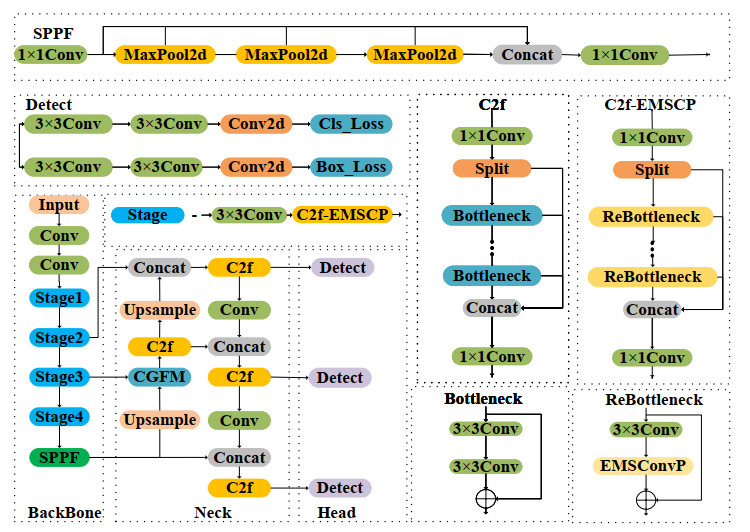
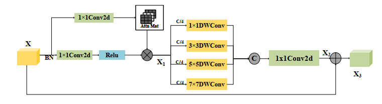
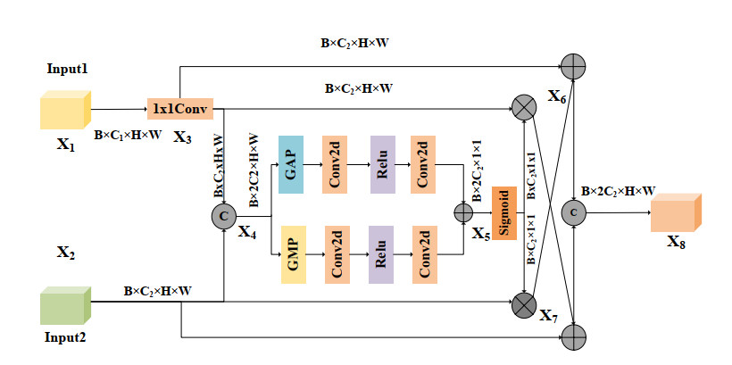
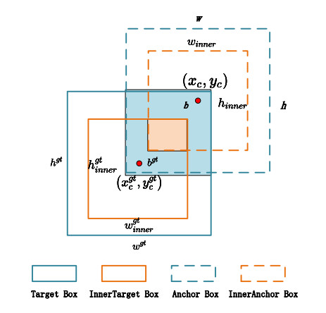
Synthetic aperture radar (SAR) is an advanced microwave sensor widely used in ocean monitoring because of its resilience to light and weather conditions. However, SAR ship detection tends to have relatively low accuracy due to the prevalence of complex backgrounds and small targets in the detection process. To address these issues, we proposed ECF-YOLO, an improved ship detection algorithm based on YOLOv8. The algorithm enhanced the feature extraction ability of the model and reduced the number of parameters and computational cost by developing a novel C2f-EMSCP module, which replaced the original C2f module in the backbone network. Additionally, we proposed the CGFM module in the neck network, which was designed to improve the detection accuracy of small ship targets by selecting features after combining shallow and deep feature maps. Furthermore, the Inner-SIoU loss function was introduced to replace the CIoU, providing a more precise overlap calculation between the target and anchor boxes, thus further improving detection accuracy. The experimental results for the SAR ship detection dataset showed that compared to YOLOv8n, ECF-YOLO improved $ \mathrm{AP_{75}} $ by 2.8% and $ \mathrm{AP_{50:95}} $ by 0.9%. Compared to other mainstream algorithms like YOLOv9t, YOLOv10n, and YOLO11n, ECF-YOLO achieved improvements of 3.4%, 4.6%, and 4.9% for $ \mathrm{AP_{75}} $, and 3.4%, 1.9%, 3.0% for $ \mathrm{AP_{50:95}} $, respectively, demonstrating its effectiveness for detecting small targets.
- YOLOv8,
- ship detection,
- C2f-EMSCP,
- CGFM,
- Inner-SIoU loss function
Citation: Peng Lu, Xinpeng Hao, Wenhui Li, Congqin Yi, Ru Kong, Teng Wang. ECF-YOLO: An enhanced YOLOv8 algorithm for ship detection in SAR images[J]. Electronic Research Archive, 2025, 33(5): 3394-3409. doi: 10.3934/era.2025150

Related Papers:

Abstract

Synthetic aperture radar (SAR) is an advanced microwave sensor widely used in ocean monitoring because of its resilience to light and weather conditions. However, SAR ship detection tends to have relatively low accuracy due to the prevalence of complex backgrounds and small targets in the detection process. To address these issues, we proposed ECF-YOLO, an improved ship detection algorithm based on YOLOv8. The algorithm enhanced the feature extraction ability of the model and reduced the number of parameters and computational cost by developing a novel C2f-EMSCP module, which replaced the original C2f module in the backbone network. Additionally, we proposed the CGFM module in the neck network, which was designed to improve the detection accuracy of small ship targets by selecting features after combining shallow and deep feature maps. Furthermore, the Inner-SIoU loss function was introduced to replace the CIoU, providing a more precise overlap calculation between the target and anchor boxes, thus further improving detection accuracy. The experimental results for the SAR ship detection dataset showed that compared to YOLOv8n, ECF-YOLO improved $ \mathrm{AP_{75}} $ by 2.8% and $ \mathrm{AP_{50:95}} $ by 0.9%. Compared to other mainstream algorithms like YOLOv9t, YOLOv10n, and YOLO11n, ECF-YOLO achieved improvements of 3.4%, 4.6%, and 4.9% for $ \mathrm{AP_{75}} $, and 3.4%, 1.9%, 3.0% for $ \mathrm{AP_{50:95}} $, respectively, demonstrating its effectiveness for detecting small targets.

References

[1]	Z. Sun, X. Leng, Y. Lei, B. Xiong, K. Ji, G. Kuang, BiFA-YOLO: A novel YOLO-based method for arbitrary-oriented ship detection in high-resolution SAR images, Remote Sens., 13 (2021), 4209. https://doi.org/10.3390/RS13214209 doi: 10.3390/RS13214209
[2]	H. Li, W. Hong, Y. Wu, P. Fan, An efficient and flexible statistical model based on generalized gamma distribution for amplitude SAR images, IEEE Trans. Geosci. Remote Sens., 48 (2010), 2711–2722. https://doi.org/10.1109/TGRS.2010.2041239 doi: 10.1109/TGRS.2010.2041239
[3]	A. Achim, E. E. Kuruoglu, J. Zerubia, SAR image filtering based on the heavy-tailed Rayleigh model, IEEE Trans. Image Process., 15 (2006), 2686–2693. https://doi.org/10.1109/TIP.2006.877362 doi: 10.1109/TIP.2006.877362
[4]	A. Breloy, G. Ginolhac, F. Pascal, P. Forster, CFAR property and robustness of the lowrank adaptive normalized matched filters detectors in low rank compound Gaussian context, in 2014 IEEE 8th Sensor Array and Multichannel Signal Processing Workshop (SAM), (2014), 301–304. https://doi.org/10.1109/SAM.2014.6882401
[5]	J. Li, C. Xu, H. Su, L. Gao, T. Wang, Deep learning for SAR ship detection: Past, present and future, Remote Sens., 14 (2022), 2712. https://doi.org/10.3390/RS14112712 doi: 10.3390/RS14112712
[6]	S. Ren, K. He, R. Girshick, J. Sun, Faster R-CNN: Towards real-time object detection with region proposal networks, IEEE Trans. Pattern Anal. Mach. Intell., 39 (2017), 1137–1149. https://doi.org/10.1109/TPAMI.2016.2577031 doi: 10.1109/TPAMI.2016.2577031
[7]	K. He, G. Gkioxari, P. Dollár, R. Girshick, Mask R-CNN, in 2017 IEEE International Conference on Computer Vision (ICCV), (2017), 2980–2988. https://doi.org/10.1109/ICCV.2017.322
[8]	Z. Cai, N. Vasconcelos, Cascade R-CNN: High quality object detection and instance segmentation, IEEE Trans. Pattern Anal. Mach. Intell., 43 (2021), 1483–1498. https://doi.org/10.1109/TPAMI.2019.2956516 doi: 10.1109/TPAMI.2019.2956516
[9]	L. Jiao, F. Zhang, F. Liu, S. Yang, L. Li, Z. Feng, et al., A survey of deep learning-based object detection, IEEE Access, 7 (2019), 128837–128868. https://doi.org/10.1109/ACCESS.2019.2939201 doi: 10.1109/ACCESS.2019.2939201
[10]	W. Liu, D. Anguelov, D. Erhan, C. Szegedy, S. Reed, C. Fu, et al., SSD: Single shot multibox detector, in Computer Vision-ECCV 2016, 9905 (2016), 21–37. https://doi.org/10.1007/978-3-319-46448-0_2
[11]	T. Lin, P. Goyal, R. Girshick, K. He, P. Dollár, Focal loss for dense object detection, IEEE Trans. Pattern Anal. Mach. Intell., 42 (2020), 318–327. https://doi.org/10.1109/TPAMI.2018.2858826 doi: 10.1109/TPAMI.2018.2858826
[12]	S. Bhattacharjee, P. Shanmugam, S. Das, A deep-learning-based lightweight model for ship localizations in SAR images, IEEE Access, 11 (2023), 94415–94427. https://doi.org/10.1109/ACCESS.2023.3310539 doi: 10.1109/ACCESS.2023.3310539
[13]	K. De Sousa, G. Pilikos, M. Azcueta, N. Floury, Ship detection from raw SAR echoes using convolutional neural networks, IEEE J. Sel. Top. Appl. Earth Obs. Remote Sens., 17 (2024), 9936–9944. https://doi.org/10.1109/JSTARS.2024.3399021 doi: 10.1109/JSTARS.2024.3399021
[14]	M. F. Humayun, F. A. Nasir, F. A. Bhatti, M. Tahir, K. Khurshid, YOLO-OSD: Optimized ship detection and localization in multiresolution SAR satellite images using a hybrid data-model centric approach, IEEE J. Sel. Top. Appl. Earth Obs. Remote Sens., 17 (2024), 5345–5363. https://doi.org/10.1109/JSTARS.2024.3365807 doi: 10.1109/JSTARS.2024.3365807
[15]	X. Tang, J. Zhang, Y. Xia, H. Xiao, DBW-YOLO: A high-precision SAR ship detection method for complex environments, IEEE J. Sel. Top. Appl. Earth Obs. Remote Sens., 17 (2024), 7029–7039. https://doi.org/10.1109/JSTARS.2024.3376558 doi: 10.1109/JSTARS.2024.3376558
[16]	J. Shen, L. Bai, Y. Zhang, M. C. Momi, S. Quan, Z. Ye, ELLK-Net: An efficient lightweight large kernel network for SAR ship detection, IEEE Trans. Geosci. Remote Sens., 62 (2024), 1–14. https://doi.org/10.1109/TGRS.2024.3451399 doi: 10.1109/TGRS.2024.3451399
[17]	S. Zhao, Z. Zhang, W. Guo, Y. Luo, An automatic ship detection method adapting to different satellites SAR images with feature alignment and compensation loss, IEEE Trans. Geosci. Remote Sens., 60 (2022), 1–17. https://doi.org/10.1109/TGRS.2022.3160727 doi: 10.1109/TGRS.2022.3160727
[18]	S. Zhao, Y. Zhang, Y. Luo, Y. Kang, H. Wang, Dynamically self-training open set domain adaptation classification method for heterogeneous SAR image, IEEE Geosci. Remote Sens. Lett., 21 (2024), 1–5. https://doi.org/10.1109/LGRS.2024.3360006 doi: 10.1109/LGRS.2024.3360006
[19]	GitHub, Ultralytics, 2023. Available from: https://github.com/ultralytics/ultralytics.
[20]	K. Han, Y. Wang, Q. Tian, J. Guo, C. Xu, C. Xu, GhostNet: More features from cheap operations, in 2020 IEEE/CVF Conference on Computer Vision and Pattern Recognition (CVPR), (2020), 1577–1586. https://doi.org/10.1109/CVPR42600.2020.00165
[21]	D. Qin, C. Leichner, M. Delakis, M. Fornoni, S. Luo, F. Yang, et al., MobileNetV4: Universal models for the mobile ecosystem, in Computer Vision-ECCV 2024, 15098 (2024), 78–96. https://doi.org/10.1007/978-3-031-73661-2_5
[22]	Y. Li, J. Hu, Y. Wen, G. Evangelidis, K. Salahi, Y. Wang, et al., Rethinking vision transformers for MobileNet size and speed, in Proceedings of the IEEE/CVF International Conference on Computer Vision (ICCV), (2023), 16889–16900.
[23]	H. Zhang, C. Xu, S. Zhang, Inner-IoU: More effective intersection over union loss with auxiliary bounding box, preprint, arXiv: 2311.02877.
[24]	T. Zhang, X. Zhang, J. Li, X. Xu, B. Wang, X. Zhan, et al., SAR ship detection dataset (SSDD): Official release and comprehensive data analysis, Remote Sens., 13 (2021), 3690. https://doi.org/10.3390/RS13183690 doi: 10.3390/RS13183690
[25]	J. Li, C. Qu, J. Shao, Ship detection in SAR images based on an improved faster R-CNN, in 2017 SAR in Big Data Era: Models, Methods and Applications (BIGSARDATA), (2017), 1–6. https://doi.org/10.1109/BIGSARDATA.2017.8124934
[26]	Z. Chen, K. Chen, W. Lin, J. See, H. Yu, Y. Ke, et al., PIoU Loss: Towards accurate oriented object detection in complex environments, in Computer Vision-ECCV 2020, 12350 (2020), 195–211. https://doi.org/10.1007/978-3-030-58558-7_12
[27]	Z. Zheng, P. Wang, W. Liu, J. Li, R. Ye, D. Ren, Distance-IoU Loss: Faster and better learning for bounding box regression, in Proceedings of the AAAI Conference on Artificial Intelligence, 34 (2020), 12993–13000. https://doi.org/10.1609/AAAI.V34I07.6999
[28]	Z. Zheng, P. Wang, D. Ren, W. Liu, R. Ye, Q. Hu, et al., Enhancing geometric factors in model learning and inference for object detection and instance segmentation, IEEE Trans. Cybern., 52 (2022), 8574–8586. https://doi.org/10.1109/TCYB.2021.3095305 doi: 10.1109/TCYB.2021.3095305
[29]	H. Rezatofighi, N. Tsoi, J. Gwak, A. Sadeghian, I. Reid, S. Savarese, Generalized intersection over union: A metric and a loss for bounding box regression, in 2019 IEEE/CVF Conference on Computer Vision and Pattern Recognition (CVPR), (2019), 658–666. https://doi.org/10.1109/CVPR.2019.00075
[30]	Z. Gevorgyan, SIoU Loss: More powerful learning for bounding box regression, preprint, arXiv: 2205.12740.
[31]	S. Ma, Y. Xu, MPDIoU: A loss for efficient and accurate bounding box regression, preprint, arXiv: 2307.07662.
[32]	H. Zhang, S. Zhang, Shape-IoU: More accurate metric considering bounding box shape and scale, preprint, arXiv: 2312.17663.
[33]	C. Wang, A. Bochkovskiy, H. M. Liao, YOLOv7: Trainable bag-of-freebies sets new state-of-the-art for real-time object detectors, in 2023 IEEE/CVF Conference on Computer Vision and Pattern Recognition (CVPR), (2023), 7464–7475. https://doi.org/10.1109/CVPR52729.2023.00721
[34]	C. Feng, Y. Zhong, Y. Gao, M. R. Scott, W. Huang, TOOD: Task-aligned one-stage object detection, in 2021 IEEE/CVF International Conference on Computer Vision (ICCV), (2021), 3490–3499. https://doi.org/10.1109/ICCV48922.2021.00349
[35]	A. Wang, H. Chen, L. Liu, K. Chen, Z. Lin, J. Han, et al., YOLOv10: Real-time end-to-end object detection, preprint, arXiv: 2405.14458.
[36]	Z. Ge, S. Liu, F. Wang, Z. Li, J. Sun, YOLOX: Exceeding YOLO series in 2021, preprint, arXiv: 2107.08430.
[37]	C. Wang, I. Yeh, H. M. Liao, YOLOv9: Learning what you want to learn using programmable gradient information, in Computer Vision-ECCV 2024, 15089 (2024), 1–21. https://doi.org/10.1007/978-3-031-72751-1_1
[38]	Y. Tian, Q. Ye, D. Doermann, YOLOv12: Attention-centric real-time object detectors, preprint, arXiv: 2502.12524.
[39]	Y. Zhao, W. Lv, S. Xu, J. Wei, G. Wang, Q. Dang, et al., DETRs beat YOLOs on real-time object detection, in 2024 IEEE/CVF Conference on Computer Vision and Pattern Recognition (CVPR), (2024), 16965–16974. https://doi.org/10.1109/CVPR52733.2024.01605

Reader Comments

Your name:*

Email:*
© 2025 the Author(s), licensee AIMS Press. This is an open access article distributed under the terms of the Creative Commons Attribution License (http://creativecommons.org/licenses/by/4.0)