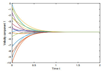
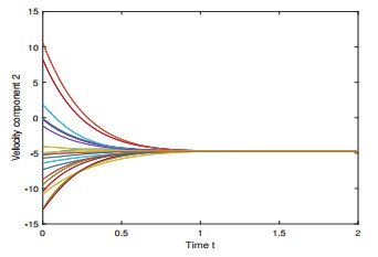
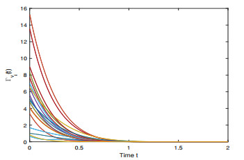
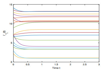
In this paper, we propose a finite-time flocking particle model with nonlinear velocity coupling and inter-driving forces. Initially, we demonstrate that under specific initial conditions, the system achieves flocking within a finite timeframe, with all particles' velocities converging to the average of their initial velocities. Our results include some results in the literature. Furthermore, a special case of mutual driving is given. Finally, we validate the obtained results through numerical simulations to confirm their accuracy.
Citation: Shixuan Zhang, Jianbo Yuan. Finite-time flocking of particle models with nonlinear velocity coupling and inter-driving forces[J]. Electronic Research Archive, 2025, 33(5): 3410-3430. doi: 10.3934/era.2025151
In this paper, we propose a finite-time flocking particle model with nonlinear velocity coupling and inter-driving forces. Initially, we demonstrate that under specific initial conditions, the system achieves flocking within a finite timeframe, with all particles' velocities converging to the average of their initial velocities. Our results include some results in the literature. Furthermore, a special case of mutual driving is given. Finally, we validate the obtained results through numerical simulations to confirm their accuracy.

| [1] |
I. D. Couzin, J. Krause, N. R. Franks, S. A. Levin, Effective leadership and decision-making in animal groups on the move, Nature, 433 (2005), 513–516. https://doi.org/10.1038/nature03236 doi: 10.1038/nature03236

|
| [2] |
M. R. D'Orsogna, Y. L. Chuang, A. L. Bertozzi, L. S. Chayes, Self-propelled particles with soft-core interactions: Patterns, stability, and collapse, Phys. Rev. Lett., 96 (2006), 104302. https://doi.org/10.1103/PhysRevLett.96.104302 doi: 10.1103/PhysRevLett.96.104302
|
| [3] |
Y. Liu, K. M. Passino, Stable social foraging swarms in a noisy environment, IEEE Trans. Autom. Control, 49 (2004), 30–44. https://doi.org/10.1109/tac.2003.821416 doi: 10.1109/tac.2003.821416
|
| [4] |
A. Jadbabaie, J. Lin, A. S. Morse, Coordination of groups of mobile autonomous agents using nearest neighbor rules, IEEE Trans. Autom. Control, 48 (2003), 988–1001. https://doi.org/10.1109/tac.2003.812781 doi: 10.1109/tac.2003.812781
|
| [5] |
H. Levine, W. J. Rappel, I. Cohen, Self-organization in systems of self-propelled particles, Phys. Rev. E, 63 (2000), 017101. https://doi.org/10.1103/PhysRevE.63.017101 doi: 10.1103/PhysRevE.63.017101
|
| [6] |
T. Vicsek, A. Czirók, E. Ben-Jacob, I. Cohen, O. Shochet, Novel type of phase transition in a system of self-driven particles, Phys. Rev. Lett., 75 (1996), 1226. https://doi.org/10.1103/PhysRevLett.75.1226 doi: 10.1103/PhysRevLett.75.1226
|
| [7] |
F. Cucker, S. Smale, Emergent behavior in flocks, IEEE Trans. Autom. Control, 52 (2007), 852–862. https://doi.org/10.1109/TAC.2007.895842 doi: 10.1109/TAC.2007.895842
|
| [8] |
F. Cucker, S. Smale, On the mathematics of emergence, Jpn. J. Math., 2 (2007), 197–227. https://doi.org/10.1007/s11537-007-0647-x doi: 10.1007/s11537-007-0647-x
|
| [9] |
S. Y. Ha, J. G. Liu, A simple proof of the Cucker-Smale flocking dynamics and mean-field limit, Commun. Math. Sci., 7 (2009), 297–325. https://doi.org/10.4310/CMS.2009.v7.n2.a2 doi: 10.4310/CMS.2009.v7.n2.a2
|
| [10] |
J. Shen, Cucker-Smale flocking under hierarchical leadership, SIAM J. Appl. Math., 68 (2008), 694–719. https://doi.org/10.1137/060673254 doi: 10.1137/060673254
|
| [11] |
Z. C. Li, X. P. Xue, Cucker-Smale flocking under rooted leadership with fixed and switching topologies, SIAM J. Appl. Math., 70 (2010), 3156–3174. https://doi.org/10.1137/100791774 doi: 10.1137/100791774
|
| [12] | Z. C. Li, S. Y. Ha, X. P. Xue, Emergent phenomena in an ensemble of Cucker-Smale particles under joint rooted leadership Math. Models Methods Appl. Sci., 24 (2014), 1389–1419. https://doi.org/10.1142/S0218202514500043 |
| [13] |
L. N. Ru, Z. C. Li, X. P. Xue, Cucker-Smale flocking with randomly failed interactions, J. Franklin Inst., 352 (2015), 1099–1118. https://doi.org/10.1016/j.jfranklin.2014.12.007 doi: 10.1016/j.jfranklin.2014.12.007
|
| [14] |
L. N. Ru, X. P. Xue, Multi-cluster flocking behavior of the hierarchical Cucker-Smale model, J. Franklin Inst., 354 (2017), 2371–2392. https://doi.org/10.1016/j.jfranklin.2016.12.018 doi: 10.1016/j.jfranklin.2016.12.018
|
| [15] |
J. G. Dong, L. Qiu, Flocking of the Cucker-Smale model on general digraphs, IEEE Trans. Autom. Control, 62 (2016), 5234–5239. https://doi.org/10.1109/TAC.2016.2631608 doi: 10.1109/TAC.2016.2631608
|
| [16] |
F. Cucker, J. G. Dong, Avoiding collisions in flocks, IEEE Trans. Autom. Control, 55 (2010), 1238–1243. https://doi.org/10.1109/TAC.2010.2042355 doi: 10.1109/TAC.2010.2042355
|
| [17] | S. Y. Ha, T. Ha, J. H. Kim, Emergent behavior of a Cucker-Smale type particle model with nonlinear velocity couplings AIMS Math., 55 (2010), 1679–1683. https://doi.org/10.1109/TAC.2010.2046113 |
| [18] |
Y. C. Liu, J. Wu, Flocking and asymptotic velocity of the Cucker-Smale model with processing delay, J. Math. Anal. Appl., 415 (2014), 53–61. https://doi.org/10.1016/j.jmaa.2014.01.036 doi: 10.1016/j.jmaa.2014.01.036
|
| [19] |
X. Wang, L. Wang, J. H. Wu, Impacts of time delay on flocking dynamics of a two-agent flock model, Commun. Nonlinear Sci. Numer. Simul., 70 (2019), 80–88. https://doi.org/10.1016/j.cnsns.2018.10.017 doi: 10.1016/j.cnsns.2018.10.017
|
| [20] |
S. Y. Ha, J. Kim, T. Ruggeri, Emergent behaviors of thermodynamic Cucker-Smale particles, SIAM J. Appl. Math., 50 (2018), 3092–3121. https://doi.org/10.1137/17M111064X doi: 10.1137/17M111064X
|
| [21] |
S. Y. Ha, T. Ruggeri, Emergent dynamics of a thermodynamically consistent particle model, Arch. Ration. Mech. Anal., 223 (2017), 1397–1425. https://doi.org/10.1007/s00205-016-1062-3 doi: 10.1007/s00205-016-1062-3
|
| [22] |
J. Zhang, J. Huang, Convergence rates and central limit theorem for 3-D stochastic fractional Boussinesq equations with transport noise, Phys. D, 470 (2027), 134406. https://doi.org/10.1016/j.physd.2024.134406 doi: 10.1016/j.physd.2024.134406
|
| [23] |
Y. C. Han, D. H. Zhao, Y. Z. Sun, Finite-time flocking problem of a Cucker-smale-type self-propelled particle model, Complexity, 21 (2016), 354–361. https://doi.org/10.1002/cplx.21747 doi: 10.1002/cplx.21747
|
| [24] | G. H. Hardy, J. E. Littlewood, G. Pólya, Inequalities, Cambridge University Press, 1952. |
| [25] |
J. Zhang, Z. Xie, Y. Xie, Long-time behavior of nonclassical diffusion equations with memory on time-dependent spaces, Asymptotic Anal., 137 (2024), 267–289. https://doi.org/10.3233/ASY-231887 doi: 10.3233/ASY-231887
|
| [26] |
J. Zhang, Z. Liu, J. Huang, Upper semicontinuity of pullback $\mathscr{D}$-attractors for nonlinear parabolic equation with nonstandard growth condition, Math. Nachr., 296 (2023), 5593–5616. https://doi.org/10.1002/mana.202100527 doi: 10.1002/mana.202100527
|
| [27] |
S. Motsch, E. Tadmor, A new model for self-organized dynamics and its flocking behavior, J. Stat. Phys., 144 (2011), 923–947. https://doi.org/10.1007/s10955-011-0285-9 doi: 10.1007/s10955-011-0285-9
|
| [28] |
S. Motsch, E. Tadmor, Heterophilious dynamics enhances consensus, SIAM Rev., 56 (2014), 577–621. https://doi.org/10.1137/120901866 doi: 10.1137/120901866
|
Figures(5)
Shixuan Zhang, Jianbo Yuan. Finite-time flocking of particle models with nonlinear velocity coupling and inter-driving forces[J]. Electronic Research Archive, 2025, 33(5): 3410-3430. doi: 10.3934/era.2025151


 DownLoad: