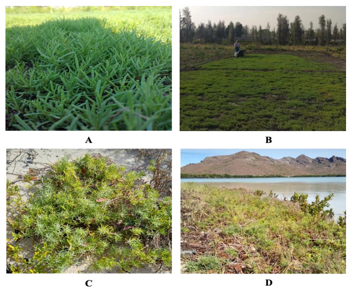
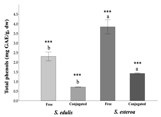
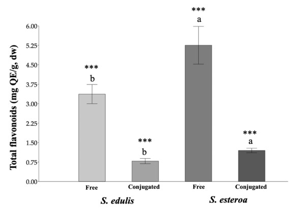
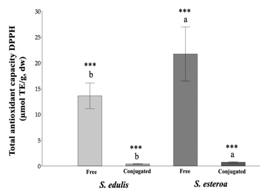
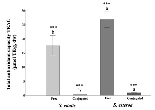
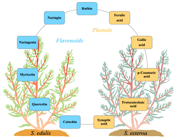
Food security is relevant due to the uncertain availability of healthy food. Accordingly, it is necessary to know the biological potential of new crops as a food source to meet the basic nutritional needs of a growing population. This study aimed to analyze chemical extractions of the cultivated species Suaeda edulis and its wild relative S. esteroa to determine their biological and nutritional value. For analysis, we collected 25 plants of S. edulis in the chinampas-producing area of Xochimilco, Mexico City, and 25 plants of S. esteroa in Balandra beach, Baja California Sur, Mexico. We quantified total phenols, total flavonoids, and the total antioxidant capacity of free and conjugated fractions by Folin-Ciocalteu, aluminum trichloride, DPPH, and TEAC spectrophotometric methods. S. esteroa reflected a higher content of total phenols, total flavonoids, and total antioxidant capacity (free and conjugated) than the values of S. edulis. We determined 39.94 and 49.64% higher values of total phenol content in S. esteroa than S. edulis, 36 and 40.33% in total flavonoid content, 32.92 and 40.50% in total antioxidant capacity by DPPH, and 34.45 and 48.91% by TEAC for free and conjugated fractions, respectively. We identified 11 phenolic compounds in both halophytes; among them, the free form ferulic acid, gallic acid, and rutin showed high concentrations in S. edulis, whereas quercetin and ferulic acid were more abundant in S. esteroa. The conjugated fraction showed lower concentrations than the free fraction. In conclusion, we found a high biologically active potential of the halophytes studied; this could boost their consumption, which in turn would offer S. edulis and S. esteroa as new sustainable crops to help address food shortages in regions with water scarcity or soil salinity, as well as to counteract chronic degenerative diseases associated with obesity.
Citation: Francyelli Regina Costa-Becheleni, Enrique Troyo-Diéguez, Alan Amado Ruiz-Hernández, Fernando Ayala-Niño, Luis Alejandro Bustamante-Salazar, Alfonso Medel-Narváez, Raúl Octavio Martínez-Rincón, Rosario Maribel Robles-Sánchez. Determination of bioactive compounds and antioxidant capacity of the halophytes Suaeda edulis and Suaeda esteroa (Chenopodiaceae): An option as novel healthy agro-foods[J]. AIMS Agriculture and Food, 2024, 9(3): 716-742. doi: 10.3934/agrfood.2024039
Food security is relevant due to the uncertain availability of healthy food. Accordingly, it is necessary to know the biological potential of new crops as a food source to meet the basic nutritional needs of a growing population. This study aimed to analyze chemical extractions of the cultivated species Suaeda edulis and its wild relative S. esteroa to determine their biological and nutritional value. For analysis, we collected 25 plants of S. edulis in the chinampas-producing area of Xochimilco, Mexico City, and 25 plants of S. esteroa in Balandra beach, Baja California Sur, Mexico. We quantified total phenols, total flavonoids, and the total antioxidant capacity of free and conjugated fractions by Folin-Ciocalteu, aluminum trichloride, DPPH, and TEAC spectrophotometric methods. S. esteroa reflected a higher content of total phenols, total flavonoids, and total antioxidant capacity (free and conjugated) than the values of S. edulis. We determined 39.94 and 49.64% higher values of total phenol content in S. esteroa than S. edulis, 36 and 40.33% in total flavonoid content, 32.92 and 40.50% in total antioxidant capacity by DPPH, and 34.45 and 48.91% by TEAC for free and conjugated fractions, respectively. We identified 11 phenolic compounds in both halophytes; among them, the free form ferulic acid, gallic acid, and rutin showed high concentrations in S. edulis, whereas quercetin and ferulic acid were more abundant in S. esteroa. The conjugated fraction showed lower concentrations than the free fraction. In conclusion, we found a high biologically active potential of the halophytes studied; this could boost their consumption, which in turn would offer S. edulis and S. esteroa as new sustainable crops to help address food shortages in regions with water scarcity or soil salinity, as well as to counteract chronic degenerative diseases associated with obesity.

| [1] | WHO (World Health Organization) (2024) Available from: https://www.who.int/health-topics/obesity#tab = tab_2. |
| [2] |
Čolak E, Pap D (2021) The role of oxidative stress in the development of obesity and obesity-related metabolic disorders. J Med Biochem 40: 1–9. https://doi.org/10.5937/jomb0-24652 doi: 10.5937/jomb0-24652

|
| [3] |
Mahmoud AM (2022) An overview of epigenetics in obesity: The role of lifestyle and therapeutic interventions. J Mol Sci 23: 1341. https://doi.org/10.3390/ijms23031341 doi: 10.3390/ijms23031341
|
| [4] | Ylli D, Sidhu S, Parikh T, et al. (2022) Endocrine changes in obesity. Endotext[Internet]. Available from: https://www.ncbi.nlm.nih.gov/books/NBK279053/. |
| [5] |
Lee CJ, Sears CL, Maruthur N (2020) Gut microbiome and its role in obesity and insulin resistance. Ann N Y Acad Sci 1461: 37–52. https://doi.org/10.1111/nyas.14107 doi: 10.1111/nyas.14107
|
| [6] |
Aziz T, Hussain N, Hameed Z, et al. (2024) Elucidating the role of diet in maintaining gut health to reduce the risk of obesity, cardiovascular and other age-related inflammatory diseases: recent challenges and future recommendations. Gut Microbes 16: 2297864. https://doi.org/10.1080/19490976.2023.2297864 doi: 10.1080/19490976.2023.2297864
|
| [7] |
Alruwaili H, Dehestani B, le Roux CW (2021) Clinical impact of liraglutide as a treatment of obesity. Clin Pharmacol: Adv and Appl 13: 53–60. https://doi.org/10.2147/CPAA.S276085 doi: 10.2147/CPAA.S276085
|
| [8] |
Huang PF, Wang QY, Chen RB, et al. (2024) A new strategy for obesity treatment: Revealing the frontiers of anti-obesity medications. Curr Mol Med 2024: 1–14. https://doi.org/10.2174/0115665240270426231123155924 doi: 10.2174/0115665240270426231123155924
|
| [9] |
Ray A, Stelloh C, Liu Y, et al. (2024) Histone modifications and their contributions to hypertension. Hypertens 81: 229–239. https://doi.org/10.1161/HYPERTENSIONAHA.123.21755 doi: 10.1161/HYPERTENSIONAHA.123.21755
|
| [10] |
Rathod P, Yadav RP (2024) Gut microbiome as therapeutic target for diabesity management: Opportunity for nanonutraceuticals and associated challenges. Drug Delv Transl Res 14: 17–29. https://doi.org/10.1007/s13346-023-01404-w doi: 10.1007/s13346-023-01404-w
|
| [11] |
Ayed K, Nabi L, Akrout R, et al. (2023) Obesity and cancer: focus on leptin. Mol Biol Rep 50: 6177–6189. https://doi.org/10.1007/s11033-023-08525-y11 doi: 10.1007/s11033-023-08525-y11
|
| [12] |
Kumar N, Goel N (2019) Phenolic acids: Natural versatile molecules with promising therapeutic applications. Biotechnol Rep 24: e00370. https://doi.org/10.1016/j.btre.2019.e00370 doi: 10.1016/j.btre.2019.e00370
|
| [13] |
Rudrapal M, Khairnar SJ, Khan J, et al. (2022) Dietary polyphenols and their role in oxidative stress-induced human diseases: Insights into protective effects, antioxidant potentials and mechanism (s) of action. Front Pharmacol 13: 283. https://doi.org/10.3389/fphar.2022.806470 doi: 10.3389/fphar.2022.806470
|
| [14] |
Rodríguez-Pérez C, Segura-Carretero A, del Mar Contreras M (2019) Phenolic compounds as natural and multifunctional anti-obesity agents: A review. Crit Rev Food Sci Nutr 59: 1212–1229. https://doi.org/10.1080/10408398.2017.1399859 doi: 10.1080/10408398.2017.1399859
|
| [15] | Bento C, Gonç alves AC, Jesus F, et al. (2017) Chapter 6—Phenolic compounds: Sources, properties, and applications. In: Porter R, Parker N (Eds.), Bioactive Compounds, 271–299. |
| [16] |
Gaur G, Gä nzle MG (2023) Conversion of (poly) phenolic compounds in food fermentations by lactic acid bacteria: Novel insights into metabolic pathways and functional metabolites. Curr Res Food Sci 6: 100448. https://doi.org/10.1016/j.crfs.2023.100448 doi: 10.1016/j.crfs.2023.100448
|
| [17] |
Dantas SBS, Moraes GKA, Araujo AR, et al. (2023) Phenolic compounds and bioactive extract produced by endophytic fungus Coriolopsis rigida. Nat Prod Res 37: 2037–2042. https://doi.org/10.1080/14786419.2022.2115492 doi: 10.1080/14786419.2022.2115492
|
| [18] |
Cecchi L, Ghizzani G, Bellumori M, et al. (2023) Virgin olive oil by-product valorization: An insight into the phenolic composition of olive seed extracts from three cultivars as sources of bioactive. Molecules 28: 2776. https://doi.org/10.3390/molecules28062776 doi: 10.3390/molecules28062776
|
| [19] |
Baccouri B, Mechi D, Rajhi I, et al. (2023) Tunisian wild olive leaves: Phenolic compounds and antioxidant activity as an important step toward their valorization. Food Anal Meth 16: 436–444. https://doi.org/10.1007/s12161-022-02430-z doi: 10.1007/s12161-022-02430-z
|
| [20] | Lozoya-Pérez NE, Orona-Tamayo D, Paredes-Molina DM, et al. (2024) Chapter 28—Microalgae: A potential opportunity for proteins and bioactive compounds destined for food and health industry. In: Nadathur S, Wanasundara JPD, Scanlin L (Eds.), Sustainable Protein Sources (Second Edition), Advances for a Healthier Tomorrow, Academic Press, 581–597. https://doi.org/10.1016/B978-0-323-91652-3.00018-6 |
| [21] |
Ruiz Hernández AA, Rouzaud Sández O, Frías J, et al. (2022) Optimization of the duration and intensity of UV-A radiation to obtain the highest free phenol content and antioxidant activity in sprouted sorghum (Sorghum bicolor L. Moench). Plants Food Hum Nutr 77: 317–318. https://doi.org/10.1007/s11130-021-00938-z doi: 10.1007/s11130-021-00938-z
|
| [22] |
Ma D, Wang C, Feng J, et al. (2021) Wheat grain phenolics: A review on composition, bioactivity, and influencing factors. J Sci Food Agric 101: 6167–6185. https://doi.org/10.1002/jsfa.11428 doi: 10.1002/jsfa.11428
|
| [23] |
Klimek-Szczykutowicz M, Prokopiuk B, Dziurka K, et al. (2022) The influence of different wavelengths of LED light on the production of glucosinolates and phenolic compounds and the antioxidant potential in in vitro cultures of Nasturtium officinale (watercress). PCTOC 149: 113–122. https://doi.org/10.1007/s11240-021-02148-6 doi: 10.1007/s11240-021-02148-6
|
| [24] |
Hassan MA, Xu T, Tian Y, et al. (2021) Health benefits and phenolic compounds of Moringa oleifera leaves: A comprehensive review. Phytomedicine 93: 153771. https://doi.org/10.1016/j.phymed.2021.153771 doi: 10.1016/j.phymed.2021.153771
|
| [25] | Flowers TJ, Hajibagheri MA, Clipson NJW (1986) Halophytes. Q Rev Biol 61: 313–337. Available from: https://www.journals.uchicago.edu/doi/abs/10.1086/415032. |
| [26] | Flowers TJ, Colmer TD (2008) Salinity tolerance in halophytes. New Phytol 179: 945–963. Available from: https://www.jstor.org/stable/25150520. |
| [27] |
Munns R, Tester M (2008) Mechanisms of salinity tolerance. Annu Rev Plant Biol 59: 651–681. https://doi.org/10.1146/annurev.arplant.59.032607.092911 doi: 10.1146/annurev.arplant.59.032607.092911
|
| [28] |
Lopes M, Sanches-Silva A, Castilho M (2023) Halophytes as source of bioactive phenolic compounds and their potential applications. Crit Rev Food Sci Nutr 63: 1078–1101. https://doi.org/10.1080/10408398.2021.1959295 doi: 10.1080/10408398.2021.1959295
|
| [29] |
Bose J, Rodrigo-Moreno A, Shabala S (2014) ROS homeostasis in halophytes in the context of salinity stress tolerance. J. Exp. Bot 65: 1241–1257. https://doi.org/10.1093/jxb/ert430 doi: 10.1093/jxb/ert430
|
| [30] | Tanveer M, Ahmed HAI (2020) ROS signaling in modulating salinity stress tolerance in plants. In: Hasanuzzaman M, Tanveer M (Eds.), Salt and Drought Stress Tolerance in Plants. Signaling and communication in plants, Springer, Cham, 229–314. https://doi.org/10.1007/978-3-030-40277-8_11 |
| [31] |
Hameed A, Ahmed MZ, Hussain T, et al. (2021) Effects of salinity stress on chloroplast structure and function. Cells 10: 2023. https://doi.org/10.3390/cells10082023 doi: 10.3390/cells10082023
|
| [32] |
Hamed KB, Ellouzi H, Talbi OZ, et al. (2013) Physiological response of halophytes to multiple stresses. Funct Plant Biol 40: 883–896. https://doi.org/10.1071/FP13074 doi: 10.1071/FP13074
|
| [33] |
Hasanuzzaman M, Raihan MRH, Masud AAC, et al. (2021) Regulation of reactive oxygen species and antioxidant defense in plants under salinity. Int J Mol Sci 22: 9326. https://doi.org/10.3390/ijms22179326 doi: 10.3390/ijms22179326
|
| [34] | Kumar S, Abedin MM, Singh AK, et al. (2020) Role of phenolic compounds in plant-defensive mechanisms. In: Lone R, Shuab R, Kamili A (Eds.), Plant Phenolics Sustainable Agriculture, Springer, Singapore, 1: 517–532. https://doi.org/10.1007/978-981-15-4890-1_22 |
| [35] |
Baysal I, Ekizoglu M, Ertas A, et al. (2021) Identification of phenolic compounds by LC-MS/MS and evaluation of bioactive properties of two edible halophytes: Limonium effusum and L. sinuatum. Molecules 26: 4040. https://doi.org/10.3390/molecules26134040 doi: 10.3390/molecules26134040
|
| [36] |
Pungin A, Lartseva L, Loskutnikova V, et al. (2023) Effect of salinity stress on phenolic compounds and antioxidant activity in halophytes Spergularia marina (L.) Griseb. and Glaux maritima L. cultured in vitro. Plants 12: 1905. https://doi.org/10.3390/plants12091905 doi: 10.3390/plants12091905
|
| [37] |
Custodio L, Garcia-Caparros P, Pereira CG, et al. (2022) Halophyte plants as potential sources of anticancer agents: A comprehensive review. Pharmaceutics 14: 2406. https://doi.org/10.3390/pharmaceutics14112406 doi: 10.3390/pharmaceutics14112406
|
| [38] |
Pereira CG, Locatelli M, Innosa D, et al. (2019) Unravelling the potential of the medicinal halophyte Eryngium maritimum L.: In vitro inhibition of diabetes-related enzymes, antioxidant potential, polyphenolic profile and mineral composition. S African J Bot 120: 204–212. https://doi.org/10.1016/j.sajb.2018.06.013 doi: 10.1016/j.sajb.2018.06.013
|
| [39] |
Cho JY, Park KH, Hwang DY, et al. (2015) Antihypertensive effects of Artemisia scoparia Waldst in spontaneously hypertensive rats and identification of angiotensin I converting enzyme inhibitors. Molecules 20: 19789–19804. https://doi.org/10.3390/molecules201119657 doi: 10.3390/molecules201119657
|
| [40] | García E (1988) Modificaciones al sistema de clasificación climática de Kö ppen. Instituto de Geografía, UNAM, México, D.F. |
| [41] |
González Carmona E, Torres Valladares CI (2014) La sustentabilidad agrícola de las chinampas en el valle de México: caso Xochimilco. Rev Mex de Agron 34: 698–709. https://doi.org/10.22004/ag.econ.173283 doi: 10.22004/ag.econ.173283
|
| [42] | Troyo Diéguez E, Mercado Mancera G, Cruz Falcón A, et al. (2014) Análisis de la sequía y desertificación mediante índices de aridez y estimación de la brecha hídrica en Baja California Sur, noroeste de México. Invest Geogr 85: 66–81. https://doi.org/10.14350/rig.32404 |
| [43] | Guevara Olivar BK, Ortega Escobar HM, Ríos Gómez R, et al. (2015) Morfología y geoquímica de suelos de Xochimilco. Terra Latinoamericana 33: 263–273. Available from: http://www.scielo.org.mx/scielo.php?script = sci_arttext & pid = S0187-57792015000400263. |
| [44] | Ferren Jr WR, Whitmore SA (1983) Suaeda esteroa (Chenopodiaceae), a new species from estuaries of Southern California and Baja California. J Calif Bot Soc Madroño 30: 181–190. Available from: https://www.jstor.org/stable/41424425. |
| [45] |
Salazar-Lopez NJ, Loarca-Piña G, Campos-Vega R, et al. (2016) The extrusion process as an alternative for improving the biological potential of sorghum bran: phenolic compounds and antiradical and anti-inflammatory capacity. Evidence-Based Complementary Altern Med 2016: 8387975. https://doi.org/10.1155/2016/8387975 doi: 10.1155/2016/8387975
|
| [46] |
Quan TH, Benjakul S, Sae-leaw T, et al. (2019) Protein–polyphenol conjugates: Antioxidant property, functionalities, and their applications. Trends Food Sci Technol 91: 507–517. https://doi.org/10.1016/j.tifs.2019.07.049 doi: 10.1016/j.tifs.2019.07.049
|
| [47] |
Adom KK, Liu RH (2002) Antioxidant activity of grains. J Agric Food Chem 50: 6182–6187. https://doi.org/10.1021/jf0205099 doi: 10.1021/jf0205099
|
| [48] |
Valenzuela-González M, Rouzaud-Sández O, Ledesma-Osuna AI, et al. (2022) Bioaccessibility of phenolic compounds, antioxidant activity, and consumer acceptability of heat-treated quinoa cookies. Food Sci Technol 42: e43421. https://doi.org/10.1590/fst.43421 doi: 10.1590/fst.43421
|
| [49] |
Ruiz-Hernández AA, Cárdenas-López JL, Cortez-Rocha MO, et al. (2021) Optimization of germination of white sorghum by response surface methodology for preparing porridges with biological potential. CyTA J Food 19: 49–55. https://doi.org/10.1080/19476337.2020.1853814 doi: 10.1080/19476337.2020.1853814
|
| [50] |
Salazar-López NJ, Astiacarán-García H, González-Aguilar GA, et al. (2017) Ferulic acid on glusose dysregulation, dyslipdemia, and inflammation in diet-induced obese rats: An integrated study. Nutrients 9: 675. https://doi.org/10.3390/nu9070675 doi: 10.3390/nu9070675
|
| [51] |
Lee KM, Kalyani D, Tiwari MK, et al. (2012) Enhanced enzymatic hydrolysis of rice straw by removal of phenolic compounds using a novel laccase from yeast Yarrowia lipolytica. Bioresour. Technol 123: 636–645. https://doi.org/10.1016/j.biortech.2012.07.066 doi: 10.1016/j.biortech.2012.07.066
|
| [52] | Social Science Statistics (2024) The Kolmogorov-Smirnov Test of Normality. Available from: https://www.socscistatistics.com/tests/kolmogorov/default.aspx. |
| [53] | Statistics Kingdom (2024) Levenexs Homocedasticity Test of Similarity of Variances. Available from: https://www.statskingdom.com/230var_levenes.html. |
| [54] | Hammer Ø, Harper, DAT, Ryan, PD (2001) PAST: Paleontological statistics software package for education and data analysis. Electron Paleontol 4: 9. Available from: https://www.nhm.uio.no/english/research/resources/past/. |
| [55] |
Agati G, Azzarello E, Pollastri S, et al. (2012) Flavonoids as antioxidants in plants: location and functional significance. Plant Sci 196: 67–76. https://doi.org/10.1016/j.plantsci.2012.07.014 doi: 10.1016/j.plantsci.2012.07.014
|
| [56] | Singh A, Roychoudhury A (2024) Role of phenolic acids and flavonoids in the mitigation of environmental stress in plants. In: Singh A, Roychoudhury A (Eds.), Biology and Biotechnology of Environmental Stress Tolerance in Plants, Apple Academica Press, 1st Edition, 22. Available from: https://www.taylorfrancis.com/chapters/edit/10.1201/9781003346173-11/role-phenolic-acids-flavonoids-mitigation-environmental-stress-plants-ankur-singh-aryadeep-roychoudhury. |
| [57] |
Zhang Y, Li Y, Ren X, et al. (2023) The positive correlation of antioxidant activity and prebiotic effect about oat phenolic compounds. Food Chem 402: 134231. https://doi.org/10.1016/j.foodchem.2022.134231 doi: 10.1016/j.foodchem.2022.134231
|
| [58] |
Kumar K, Debnath P, Singh S, et al. (2023) An overview of plant phenolics and their involvement in abiotic stress tolerance. Stresses 3: 570–585. https://doi.org/10.3390/stresses3030040 doi: 10.3390/stresses3030040
|
| [59] |
Adhikary S, Dasgupta N (2023) Role of secondary metabolites in plant homeostasis during biotic stress. Biocatal Agric Biotechnol 50: 102712. https://doi.org/10.1016/j.bcab.2023.102712 doi: 10.1016/j.bcab.2023.102712
|
| [60] |
Parada J, Aguilera JM (2007) Food microstructure affects the bioavailability of several nutrients. J Food Sci 72: R21–R32. https://doi.org/10.1111/j.1750-3841.2007.00274.x doi: 10.1111/j.1750-3841.2007.00274.x
|
| [61] |
Gao Y, Ma S, Wang M, et al. (2017) Characterization of free, conjugated, and bound phenolic acids in seven commonly consumed vegetables. Molecules 22: 1878. https://doi.org/10.3390/molecules22111878 doi: 10.3390/molecules22111878
|
| [62] |
Bautista I, Boscaiu M, Lidón A, et al. (2016) Environmentally induced changes in antioxidant phenolic compounds levels in wild plants. Acta Physiol Plant 38: 9. https://doi.org/10.1007/s11738-015-2025-2 doi: 10.1007/s11738-015-2025-2
|
| [63] |
Aloisi I, Parrotta L, Ruiz KB, et al. (2016) New insight into quinoa seed quality under salinity: Changes in proteomic and amino acid profiles, phenolic content, and antioxidant activity of protein extracts. Front Plant Sci 7: 656. https://doi.org/10.3389/fpls.2016.00656 doi: 10.3389/fpls.2016.00656
|
| [64] |
Muñoz-Bernal Ó A, Torres-Aguirre GA, Núñez-Gastélum JA, et al. (2017) Nuevo acercamiento a la interacción del reactivo de Folin-Ciocalteu con azúcares durante la cuantificación de polifenoles totals. TIP 20: 23–28. https://doi.org/10.1016/j.recqb.2017.04.003 doi: 10.1016/j.recqb.2017.04.003
|
| [65] |
Everette JD, Bryant QM, Green AM, et al. (2010) Thorough study of reactivity of various compound classes toward the Folin-Ciocalteu reagent. J Agric Food Chem 58: 8139–8144. https://doi.org/10.1021/jf1005935 doi: 10.1021/jf1005935
|
| [66] |
Liu W, Feng Y, Yu S, et al. (2021) The flavonoid biosynthesis network in plants. Int J Mol Sci 22: 12824. https://doi.org/10.3390/ijms222312824 doi: 10.3390/ijms222312824
|
| [67] |
Agati G, Brunetti C, Fini A, et al. (2020) Are flavonoids effective antioxidants in plants? Twenty years of our investigation. Antioxidants 9: 1098. https://doi.org/10.3390/antiox9111098 doi: 10.3390/antiox9111098
|
| [68] |
Dias MC, Pinto DC, Silva AM (2021) Plant flavonoids: Chemical characteristics and biological activity. Molecules 26: 5377. https://doi.org/10.3390/molecules26175377 doi: 10.3390/molecules26175377
|
| [69] | Ahmad R, Hussain S, Anjum MA, et al. (2019) Oxidative stress and antioxidant defense mechanisms in plants under salt stress. In: Hasanuzzaman M, Hakeem K, Nahar K, et al. (Eds.), Plant Abiotic Stress Tolerance: Agronomic, molecular, and biotechnological approaches, Springer, Cham, 191–205. https://doi.org/10.1007/978-3-030-06118-0_8 |
| [70] |
Marchiosi R, dos Santos WD, et al. (2020) Biosynthesis and metabolic actions of simple phenolic acids in plants. Phytochem Rev 19: 865–906. https://doi.org/10.1007/s11101-020-09689-2 doi: 10.1007/s11101-020-09689-2
|
| [71] |
Giuffrè AM (2019) Bergamot (Citrus bergamia, Risso): The effects of cultivar and harvest date on functional properties of juice and cloudy juice. Antioxidants 8: 221. https://doi.org/10.3390/antiox8070221 doi: 10.3390/antiox8070221
|
| [72] |
Deng GF, Shen C, Xu XR, et al. (2012) Potential of fruit wastes as natural resources of bioactive compounds. Int J Mol Sci 13: 8308–8323. https://doi.org/10.3390/ijms13078308 doi: 10.3390/ijms13078308
|
| [73] |
Christodoulou MC, Orellana Palacios JC, Hesami G, et al. (2022) Spectrophotometric methods for measurement of antioxidant activity in food and pharmaceuticals. Antioxidants 11: 2213. https://doi.org/10.3390/antiox11112213 doi: 10.3390/antiox11112213
|
| [74] | Bakhshi S, Abbaspour H, Saeidisar S (2018) Study of phytochemical changes, enzymatic and antioxidant activity of two halophyte plants: Salsola dendroides Pall and Limonium reniforme (Girard) Lincz in different seasons. J Plant Environ Physiol 46: 79–92. |
| [75] |
Castañeda-Loaiza V, Oliveira M, Santos T, et al. (2020) Wild vs cultivated halophytes: Nutritional and functional differences. Food Chem 333: 127536. https://doi.org/10.1016/j.foodchem.2020.127536 doi: 10.1016/j.foodchem.2020.127536
|
| [76] |
Skroza D, Šimat V, Vrdoljak L, et al. (2022) Investigation of antioxidant synergisms and antagonisms among phenolic acids in the model matrices using FRAP and ORAC methods. Antioxidants 11: 1784. https://doi.org/10.3390/antiox11091784 doi: 10.3390/antiox11091784
|
| [77] | Kutchan TM, Gershenzon J, Moller BL, et al. (2015) Natural products. In: Buchanan BB, Gruissem W, Jones RL (Eds.), Biochemistry and Molecular Biology of Plants, Wiley, New York, 1132–1205. |
| [78] |
Boerjan W, Ralph J, Baucher M (2003) Lignin biosynthesis. Annu Rev Plant Biol 54: 519–546. https://doi.org/10.1146/annurev.arplants.54.031902.134938 doi: 10.1146/annurev.arplants.54.031902.134938
|
| [79] |
Vanholme R, Demedts B, Morreel K, et al. (2010) Lignin biosynthesis and structure. Plant Physiol 153: 895–905. https://doi.org/10.1104/pp.110.155119 doi: 10.1104/pp.110.155119
|
| [80] |
Wildermuth MC (2006) Variations on a theme: synthesis and modification of plant benzoic acids. Curr Opin Plant Biol 9: 288–296. https://doi.org/10.1016/j.pbi.2006.03.006 doi: 10.1016/j.pbi.2006.03.006
|
| [81] |
Widhalm JR, Dudareva N (2015) A familiar ring to it: biosynthesis of plant benzoic acids. Mol Plant 8: 83–97. https://doi.org/10.1016/j.molp.2014.12.001 doi: 10.1016/j.molp.2014.12.001
|
| [82] | Heller W, Forkmann G (2017) Biosynthesis of flavonoids. In: Harborne JB (Ed.), The Flavonoids Advances in Research Since 1986, Routledge, 1st Edition, 37. Available from: https://www.taylorfrancis.com/chapters/edit/10.1201/9780203736692-11/biosynthesis-flavonoids-werner-heller-gert-forkmann. |
| [83] |
Mandal SM, Chakraborty D, Dey S (2010) Phenolic acids act as signaling molecules in plant-microbe symbioses. Plant Signaling Behav 5: 359–368. https://doi.org/10.4161/psb.5.4.10871 doi: 10.4161/psb.5.4.10871
|
| [84] |
Padayachee A, Netzel G, Netzel M, et al. (2012) Binding of polyphenols to plant cell wall analogues-Part 2: Phenolic acids. Food Chem 135: 2287–2292. https://doi.org/10.1016/j.foodchem.2012.07.004 doi: 10.1016/j.foodchem.2012.07.004
|
| [85] |
Hajlaoui H, Arraouadi S, Mighri H, et al. (2022) HPLC-MS profiling, antioxidant, antimicrobial, antidiabetic, and cytotoxicity activities of Arthrocnemum indicum (Willd.) Moq. extracts. Plants 11: 232. https://doi.org/10.3390/plants11020232 doi: 10.3390/plants11020232
|
| [86] |
Jdey A, Falleh H, Jannet SB, et al. (2017) Phytochemical investigation and antioxidant, antibacterial and anti-tyrosinase performances of six medicinal halophytes. S African J Bot 112: 508–514. https://doi.org/10.1016/j.sajb.2017.05.016 doi: 10.1016/j.sajb.2017.05.016
|
| [87] |
Sánchez-Gavilán I, Ramírez Chueca E, de la Fuente García V (2021) Bioactive compounds in Sarcocornia and Arthrocnemum, two wild halophilic genera from the Iberian Peninsula. Plants 10: 2218. https://doi.org/10.3390/plants10102218 doi: 10.3390/plants10102218
|
| [88] |
De Oliveira DM, Finger‐Teixeira A, Rodrigues Mota T, et al. (2014) Ferulic acid: A key component in grass lignocellulose recalcitrance to hydrolysis. Plant Biotechnol J 13: 1224–1232. https://doi.org/10.1111/pbi.12292 doi: 10.1111/pbi.12292
|
| [89] |
Buanafina MMDO, Morris P (2022) The impact of cell wall feruloylation on plant growth, responses to environmental stress, plant pathogens and cell wall degradability. Agronomy 12: 1847. https://doi.org/10.3390/agronomy12081847 doi: 10.3390/agronomy12081847
|
| [90] |
Deng Y, Feng Z, Yuan F, et al. (2015) Identification and functional analysis of the autofluorescent substance in Limonium bicolor salt glands. Plant Physiol Biochem 97: 20–27. https://doi.org/10.1016/j.plaphy.2015.09.007 doi: 10.1016/j.plaphy.2015.09.007
|
| [91] | Fitzpatrick LR, Woldemariam T (2017) Small-molecule drugs for the treatment of inflammatory bowel disease. In: Comprehensive Medicinal Chemistry III, Elsevier Inc., 495–510. |
| [92] |
Zhang X, Ran W, Li X, et al. (2022) Exogenous application of gallic acid induces the direct defense of tea plant against Ectropis obliqua caterpillars. Front Plant Sci 13: 833489. https://doi.org/10.3389/fpls.2022.833489 doi: 10.3389/fpls.2022.833489
|
| [93] | Waśkiewicz A, Muzolf-Panek M, Goliński P (2013) Phenolic content changes in plants under salt stress. In: Ahmad P, Azooz M, Prasad M (Eds.), Ecophysiology and Responses of Plants under Salt Stress, Springer, New York, 283–314. https://doi.org/10.1007/978-1-4614-4747-4_11 |
| [94] |
Singh P, Arif Y, Bajguz A, et al. (2021) The role of quercetin in plants. Plant Physiol Biochem 166: 10–19. https://doi.org/10.1016/j.plaphy.2021.05.023 doi: 10.1016/j.plaphy.2021.05.023
|
| [95] |
Agati G, Brunetti C, Di Ferdinando M, et al. (2013) Functional roles of flavonoids in photoprotection: new evidence, lessons from the past. Plant Physiol Biochem 72: 35–45. https://doi.org/10.1016/j.plaphy.2013.03.014 doi: 10.1016/j.plaphy.2013.03.014
|
| [96] |
Cesco S, Mimmo T, Tonon G, et al. (2012) Plant-borne flavonoids released into the rhizosphere: impact on soil bioactivities related to plant nutrition. A review. Biol Fertil Soils 48: 123–149. https://doi.org/10.1007/s00374-011-0653-2 doi: 10.1007/s00374-011-0653-2
|
| [97] |
Ng JLP, Hassan S, Truong TT (2015) Flavonoids and auxin transport inhibitors rescue symbiotic nodulation in the Medicago truncatula cytokinin perception mutant cre1. Plant Cell 27: 2210–2226. https://doi.org/10.1105/tpc.15.00231 doi: 10.1105/tpc.15.00231
|
| [98] |
Peer W, Blakeslee J, Yang H, et al. (2011) Seven things we think we know about auxin transport. Mol Plant 4: 487–504. https://doi.org/10.1093/mp/ssr034 doi: 10.1093/mp/ssr034
|
| [99] |
Agati G, Matteini P, Goti A, et al. (2007) Chloroplast‐located flavonoids can scavenge singlet oxygen. New Phytol 174: 77–89. https://doi.org/10.1111/j.1469-8137.2007.01986.x doi: 10.1111/j.1469-8137.2007.01986.x
|
| [100] |
Chagas MDSS, Behrens MD, Moragas-Tellis CJ, et al. (2022) Flavonols and flavones as potential anti-inflammatory, antioxidant, and antibaterial compounds. Oxid Med Cell Longevity 2022: 9966750. https://doi.org/10.1155/2022/9966750 doi: 10.1155/2022/9966750
|
| [101] | de Souza M M, da Silva B, Badiale-Furlong E, et al. (2021) Phenolic acid profile, quercetin content, and antioxidant activity of six Brazilian halophytes. In: Grigore MN (Ed.), Handbook of Halophytes: From Molecules to Ecosystems towards Biosaline Agriculture, Springer, Cham, 1395–1419. https://doi.org/10.1007/978-3-030-57635-6_44 |
| [102] |
Shomali A, Das S, Arif N, et al. (2022) Diverse physiological roles of flavonoids in plant environmental stress responses and tolerance. Plants 11: 3158. https://doi.org/10.3390/plants11223158 doi: 10.3390/plants11223158
|
| [103] | Frutos MJ, Rincón-Frutos L, Valero-Cases E (2019) Chapter 2.14—Rutin. In: Nonvitamin and Nonmineral Nutritional Supplements, Academic Press, 111–117. https://doi.org/10.1016/B978-0-12-812491-8.00015-1 |
| [104] |
Hodaei M, Rahimmalek M, Arzani A, et al. (2018) The effect of water stress on phytochemical accumulation, bioactive compounds and expression of key genes involved in flavonoid biosynthesis in Chrysanthemum morifolium L. Ind Crops Prod 120: 295–304. https://doi.org/10.1016/j.indcrop.2018.04.073 doi: 10.1016/j.indcrop.2018.04.073
|
| [105] |
Sánchez-Gavilán I, Ramírez E, de la Fuente V, et al. (2021) Bioactive compounds in Salicornia patula Duval-Jouve: A mediterranean edible euhalophyte. Foods 10: 410. https://doi.org/10.3390/foods10020410 doi: 10.3390/foods10020410
|
| [106] |
Chekroun-Bechlaghem N, Belyagoubi-Benhammou N, Belyagoubi L, et al. (2019) Phytochemical analysis and antioxidant activity of Tamarix africana, Arthrocnemum macrostachyum and Suaeda fruticosa, three halophyte species from Algeria. Plant Biosyst-Int J Deal Asp Plant Biol 153: 843–852. https://doi.org/10.1080/11263504.2018.1555191 doi: 10.1080/11263504.2018.1555191
|
| [107] |
Zeb A (2020) Concept, mechanism, and applications of phenolic antioxidants in foods. J Food Biochem 44: e13394. https://doi.org/10.1111/jfbc.13394 doi: 10.1111/jfbc.13394
|
| [108] |
Zengin G, Aumeeruddy-Elalfi Z, Mollica A, et al. (2018) In vitro and in silico perspectives on biological and phytochemical profile of three halophyte species—A source of innovative phytopharmaceuticals from nature. Phytomedicine 38: 35–44. https://doi.org/10.1016/j.phymed.2017.10.017 doi: 10.1016/j.phymed.2017.10.017
|
| [109] |
Vilela C, Santos SA, Coelho D, et al. (2014) Screening of lipophilic and phenolic extractives from different morphological parts of Halimione portulacoides. Ind Crops Prod 52: 373–379. https://doi.org/10.1016/j.indcrop.2013.11.002 doi: 10.1016/j.indcrop.2013.11.002
|
| [110] | Stanković M, Jakovljević D (2021) Phytochemical diversity of halophytes. In: Grigore MN (Ed.), Handbook of Halophytes, Springer, Cham, 2089–2114. https://doi.org/10.1007/978-3-030-57635-6_125 |
| [111] |
Chiavaroli A, Sinan KI, Zengin G, et al. (2020) Identification of chemical profiles and biological properties of Rhizophora racemosa G. Mey. extracts obtained by different methods and solvents. Antioxidants 9: 533. https://doi.org/10.3390/antiox9060533 doi: 10.3390/antiox9060533
|
| [112] |
Cho JY, Yang X, Park KH, et al. (2013) Isolation and identification of antioxidative compounds and their activities from Suaeda japonica. Food Sci Biotechnol 22: 1547–1557. https://doi.org/10.1007/s10068-013-0250-2 doi: 10.1007/s10068-013-0250-2
|
| [113] | Pratyusha S (2022) Phenolic compounds in the plant development and defense: An overview. In: Plant stress physiology-perspectives in agriculture, 125–140. |
| [114] |
Sun R, Sun XF, Wang SQ, et al. (2002) Ester and ether linkages between hydroxycinnamic acids and lignins from wheat, rice, rye, and barley straws, maize stems, and fast-growing poplar wood. Ind Crops Prod 15: 179–188. https://doi.org/10.1016/S0926-6690(01)00112-1 doi: 10.1016/S0926-6690(01)00112-1
|
| [115] |
Ueda M, Sawai Y, Shibazaki Y, et al. (1998) Leaf-opening substance in the nyctinastic plant, Albizzia julibrissin Durazz. Biosci Biotechnol Biochem 62: 2133–2137. https://doi.org/10.1271/bbb.62.2133 doi: 10.1271/bbb.62.2133
|
| [116] |
Li ZH, Wang Q, Ruan X, et al. (2010) Phenolics and plant allelopathy. Molecules 15: 8933–8952. https://doi.org/10.3390/molecules15128933 doi: 10.3390/molecules15128933
|
| [117] |
Begum AA, Leibovitch S, Migner P, et al. (2001) Specific flavonoids induced nod gene expression and pre‐activated nod genes of Rhizobium leguminosarum increased pea (Pisum sativum L.) and lentil (Lens culinaris L.) nodulation in controlled growth chamber environments. J Exp Bot 52: 1537–1543. https://doi.org/10.1093/jexbot/52.360.1537 doi: 10.1093/jexbot/52.360.1537
|
| [118] |
Chaudhry UK, Ö ztürk ZN, Gö kç e AF (2024) Assessment of salt and drought stress on the biochemical and molecular functioning of onion cultivars. Mol Biol Rep 51: 37. https://doi.org/10.1007/s11033-023-08923-2 doi: 10.1007/s11033-023-08923-2
|
| [119] |
Ri I, Pak S, Pak U, et al. (2024) How does UV-B radiation influence the photosynthesis and secondary metabolism of Schisandra chinensis leaves?. Ind Crops Prod 208: 117832. https://doi.org/10.1016/j.indcrop.2023.117832 doi: 10.1016/j.indcrop.2023.117832
|
| [120] |
Scalzini G, Vernhet A, Carillo S, et al. (2024) Cell wall polysaccharides, phenolic extractability, and mechanical properties of Aleatico winegrapes dehydrated under sun or in controlled conditions. Food Hydrocoll 149: 109605. https://doi.org/10.1016/j.foodhyd.2023.109605 doi: 10.1016/j.foodhyd.2023.109605
|
| [121] |
Panth N, Park SH, Kim HJ, et al. (2016) Protective effect of Salicornia europaea extracts on high salt intake-induced vascular dysfunction and hypertension. Int J Mol Sci 17: 1176. https://doi.org/10.3390/ijms17071176 doi: 10.3390/ijms17071176
|
| [122] |
Nikalje GC, Srivastava AK, Pandey GK, et al. (2018) Halophytes in biosaline agriculture: Mechanism, utilization, and value addition. Land Degrad Dev 29: 1081–1095. https://doi.org/10.1002/ldr.2819 doi: 10.1002/ldr.2819
|
| [123] |
Ventura Y, Sagi M (2013) Halophyte crop cultivation: The case for Salicornia and Sarcocornia. Environ Exp Bot 92: 144–153. https://doi.org/10.1016/j.envexpbot.2012.07.010 doi: 10.1016/j.envexpbot.2012.07.010
|
| [124] |
Ventura Y, Wuddineh WA, Myrzabayeva M, et al. (2011) Effect of seawater concentration on the productivity and nutritional value of annual Salicornia and perennial Sarcocornia halophytes as leafy vegetable crops. Sci Hortic 128: 189–196. https://doi.org/10.1016/j.scienta.2011.02.001 doi: 10.1016/j.scienta.2011.02.001
|
| [125] |
Ghasemzadeh A, Ghasemzadeh N (2011) Flavonoids and phenolic acids: Role and biochemical activity in plants and human. J Med Plants Res 5: 6697–6703. https://doi.org/10.5897/JMPR11.1404 doi: 10.5897/JMPR11.1404
|
| [126] |
Ozcan T, Akpinar-Bayizit A, Yilmaz-Ersan L, et al. (2014) Phenolics in human health. Int J Chem Eng Appl 5: 5. https://doi.org/10.7763/IJCEA.2014.V5.416 doi: 10.7763/IJCEA.2014.V5.416
|
Figures(7) / Tables(4)

Francyelli Regina Costa-Becheleni, Enrique Troyo-Diéguez, Alan Amado Ruiz-Hernández, Fernando Ayala-Niño, Luis Alejandro Bustamante-Salazar, Alfonso Medel-Narváez, Raúl Octavio Martínez-Rincón, Rosario Maribel Robles-Sánchez. Determination of bioactive compounds and antioxidant capacity of the halophytes Suaeda edulis and Suaeda esteroa (Chenopodiaceae): An option as novel healthy agro-foods[J]. AIMS Agriculture and Food, 2024, 9(3): 716-742. doi: 10.3934/agrfood.2024039


 DownLoad: