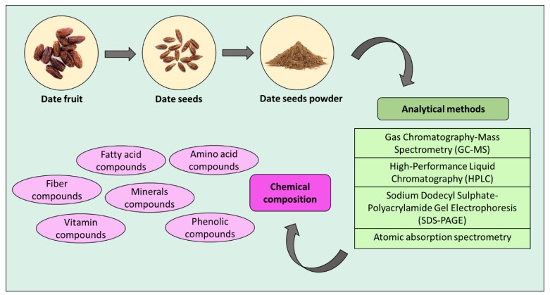
Since ancient times, date fruit has been used as a staple food because of its high nutritional value and caloric content. With the development of food science and the application of modern instrumentation, we now know that date seeds contain large amounts of dietary fiber, phenols, polyphenols, amino acids, fatty acids, and many vitamins and minerals. Due to the presence of these functional food ingredients, date seeds are used in various applications, including foods such as bread, hot beverages, cosmetics such as hair and skin products, and as feed for culturing aquatic animals. Date seeds have been used in clinical applications, making use of their antioxidant, anti-inflammatory, anti-cancer, anti-diabetic, and antimicrobial properties. There is now growing awareness of the value of date seeds, which were considered a waste product. In this review, we focused on explaining the major biochemical constituents of date seeds and developing these constituents for various applications. We also highlight the expected developments in date seed use for the future.
Citation: Asma Hussain Alkatheri, Mahra Saleh Alkatheeri, Wan-Hee Cheng, Warren Thomas, Kok-Song Lai, Swee-Hua Erin Lim. Innovations in extractable compounds from date seeds: Farms to future[J]. AIMS Agriculture and Food, 2024, 9(1): 256-281. doi: 10.3934/agrfood.2024016
Since ancient times, date fruit has been used as a staple food because of its high nutritional value and caloric content. With the development of food science and the application of modern instrumentation, we now know that date seeds contain large amounts of dietary fiber, phenols, polyphenols, amino acids, fatty acids, and many vitamins and minerals. Due to the presence of these functional food ingredients, date seeds are used in various applications, including foods such as bread, hot beverages, cosmetics such as hair and skin products, and as feed for culturing aquatic animals. Date seeds have been used in clinical applications, making use of their antioxidant, anti-inflammatory, anti-cancer, anti-diabetic, and antimicrobial properties. There is now growing awareness of the value of date seeds, which were considered a waste product. In this review, we focused on explaining the major biochemical constituents of date seeds and developing these constituents for various applications. We also highlight the expected developments in date seed use for the future.

| [1] |
Al-Okbi SY (2022) Date palm as source of nutraceuticals for health promotion: A review. Curr Nutr Rep 11: 574–591. https://doi.org/10.1007/s13668-022-00437-w doi: 10.1007/s13668-022-00437-w

|
| [2] |
Al-Dashti YA, Holt RR, Keen CL, et al. (2021) Date palm fruit (Phoenix dactylifera): Effects on vascular health and future research directions. Int J Mol Sci 22: 4665. https://doi.org/10.3390/ijms22094665 doi: 10.3390/ijms22094665
|
| [3] |
Karimi A, Elmi A, Zargaran A, et al. (2020) Clinical effects of date palm (Phoenix dactylifera L.): A systematic review on clinical trials. Complementary Ther Med 51: 102429. https://doi.org/10.1016/j.ctim.2020.102429 doi: 10.1016/j.ctim.2020.102429
|
| [4] | Rahmani AH, Aly SM, Ali H, et al. (2014) Therapeutic effects of date fruits (Phoenix dactylifera) in the prevention of diseases via modulation of anti-inflammatory, anti-oxidant and anti-tumour activity. Int J Clin Exp Med 7: 483. |
| [5] |
Marwat SK, Khan MA, Rehman, et al. (2009) Aromatic plant species mentioned in the holy Qura'n and Ahadith and their ethnomedicinal importance. Pak J Nutr 8: 1472–1479. https://doi.org/10.3923/pjn.2009.1472.1479 doi: 10.3923/pjn.2009.1472.1479
|
| [6] |
Taleb H, Maddocks SE, Morris RK, et al. (2016) Chemical characterisation and the anti-inflammatory, anti-angiogenic and antibacterial properties of date fruit (Phoenix dactylifera L.). J Ethnopharmacol 194: 457–468. https://doi.org/10.1016/j.jep.2016.10.032 doi: 10.1016/j.jep.2016.10.032
|
| [7] | Abdel S, Itimad E, Awad A (2012) Comparative study on five Sudanese date (Phoenix dactylifera L.) fruit cultivars. Food Nutr Sci 3: 22292. |
| [8] | Shahbandeh M (2023) Statista. Fruit date market. Available from: https://www.statista.com/topics/6326/fruit-date-market/. |
| [9] | Solo D (2023) Date Fruit Market 2023: Producers, Market Offerings, And End Use Outlook Ⅰ Khoshbin Group. Available from: https://ratinkhosh.com/date-fruit-market/. |
| [10] | Elsharawy N, Al-Mutarrafi M, Alayafi A (2019) Different types of dates in Saudi Arabia and its most fungal spoilage and its most preservation methods. Int J Sci Res 10: 35787–35799. |
| [11] |
Al-Farsi M, Lee C (2008) Nutritional and functional properties of dates: A review. Crit Rev Food Sci Nutr 48: 877–887. https://doi.org/10.1080/10408390701724264 doi: 10.1080/10408390701724264
|
| [12] |
Al-Shahib W, Marshall RJ (2003) The fruit of the date palm: Its possible use as the best food for the future? Int J Food Sci Nutr 54: 247–259. https://doi.org/10.1080/09637480120091982 doi: 10.1080/09637480120091982
|
| [13] | Gul F, Shinwari ZK, Afzal I (2012) Screening of indigenous knowledge of herbal remedies for skin diseases among local communities of North West Punjab, Pakistan. Pak J Bot 5: 1609–1616. |
| [14] | Kabbaj FZ, Meddah B, Cherrah Y (2019) Ethnopharmacological profile of traditional plants used in Morocco by cancer patients as herbal therapeutics. Am J Ethnomed 2: 243–256. |
| [15] |
El-Far AH, Oyinloye BE, Sepehrimanesh M, et al. (2019) Date palm (Phoenix dactylifera): Novel findings and future directions for food and drug discovery. Curr Drug Discov Technol 16: 2–10. https://doi.org/10.2174/1570163815666180320111937 doi: 10.2174/1570163815666180320111937
|
| [16] |
Alkhoori MA, Kong AS-Y, Aljaafari MN, et al. (2022) Biochemical composition and biological activities of date palm (Phoenix dactylifera L.) seeds: A review. Biomolecules 12: 1626. https://doi.org/10.3390/biom12111626 doi: 10.3390/biom12111626
|
| [17] |
Ren J, Mozurkewich EL, Sen A, et al. (2013) Total serum fatty acid analysis by GC-MS: Assay validation and serum sample stability. Curr Pharm Anal 9: 331–339. https://doi.org/10.2174/1573412911309040002 doi: 10.2174/1573412911309040002
|
| [18] |
Gao L, Xu P, Ren J (2023) A sensitive and economical method for simultaneous determination of D/L- amino acids profile in foods by HPLC-UV: Application in fermented and unfermented foods discrimination. Food Chem 410: 135382. https://doi.org/10.1016/j.foodchem.2022.135382 doi: 10.1016/j.foodchem.2022.135382
|
| [19] | Saraswathy N, Ramalingam P (2011) Phosphoproteomics. In: Saraswathy N, Ramalingam P (Eds.), Concepts and Techniques in Genomics and Proteomics, Woodhead Publishing, 203–211. https://doi.org/10.1533/9781908818058.203 |
| [20] | Slavin W (1994) Atomic absorption spectrometry Flame AAS. In: Herber RFM, Stoeppler M (Eds.), Techniques and Instrumentation in Analytical Chemistry, Elsevier, 87–90. https://doi.org/10.1016/S0167-9244(08)70146-X |
| [21] | Yu L, Choe U, Yanfang L, et al. (2020) Oils from Fruit, Spice, and Herb Seeds, 1–35. |
| [22] | Qadir A, Singh SP, Akhtar J, et al. (2018) Chemical composition of Saudi Arabian Sukkari variety of date seed oil and extracts obtained by slow pyrolysis. Indian J Pharm Sci 80: 940–946. |
| [23] | Bolla AS, Patel AR, Priefer R (2020) The silent development of counterfeit medications in developing countries—A systematic review of detection technologies. Int J Pharm 587: 119702. |
| [24] | Mrabet A, Jiménez-Araujo A, Guillén-Bejarano R, et al. (2020) Date seeds: A promising source of oil with functional properties. Foods 9: 787. |
| [25] | Murthy HN, Yadav GG, Dewir YH, et al. (2021) Phytochemicals and biological activity of desert date (Balanites aegyptiaca (L.) Delile). Plants 10: 32. |
| [26] | Bouallegue K, Allaf T, Besombes C, et al. (2019) Phenomenological modeling and intensification of texturing/grinding-assisted solvent oil extraction: case of date seeds (Phoenix dactylifera L.). Arabian J Chem 12: 2398–2410. |
| [27] | Habib HM, Kamal H, Ibrahim WH, et al. (2013) Carotenoids, fat soluble vitamins and fatty acid profiles of 18 varieties of date seed oil. Ind Crops Prod 42: 567–572. |
| [28] | AL-Kahtani HA, Abdul Rahman R, Mansor TST, et al. (2013) Date seed and date seed oil. Int Food Res J 20: 2035. |
| [29] | Alharbi KL, Raman J, Shin H-J (2021) Date fruit and seed in nutricosmetics. Cosmetics 8: 59. |
| [30] |
Kari ZA, Goh KW, Edinur HA, et al. (2022) Palm date meal as a non-traditional ingredient for feeding aquatic animals: A review. Aquacult Rep 25: 101233. https://doi.org/10.1016/j.aqrep.2022.101233 doi: 10.1016/j.aqrep.2022.101233
|
| [31] |
Bentrad N, Gaceb-Terrak R, Benmalek Y, et al. (2017) Studies on chemical composition and antimicrobial activities of bioactive molecules from date palm (Phoenix dactylifera L.) pollens and seeds. Afr J Tradit, Complementary Altern Med 14: 242–256. https://doi.org/10.21010/ajtcam.v14i3.26 doi: 10.21010/ajtcam.v14i3.26
|
| [32] | Shina S, Izuagie T, Shuaibu M, et al. (2013) The nutritional evaluation and medicinal value of date palm (Phoenix dactylifera). Int J Modern Chem 4: 147–154. |
| [33] | Sheikh DME, El-Kholany EA, Kamel SM (2014) Nutritional value, cytotoxicity, anti-carcinogenic and beverage evaluation of roasted date pits. World J Dairy Food Sci 9: 308–316. |
| [34] |
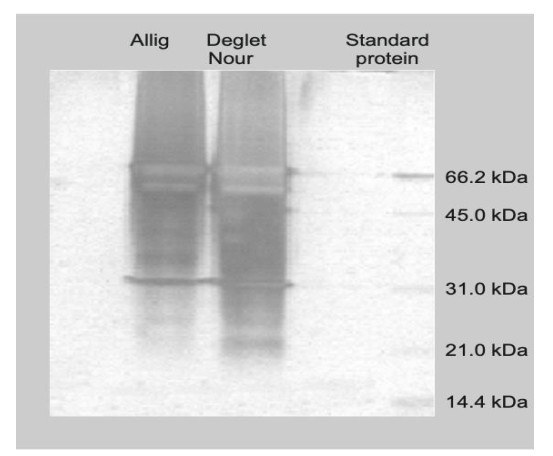
Bouaziz MA, Besbes S, Blecker C, et al. (2008) Protein and amino acid profiles of Tunisian Deglet Nour and Allig date palm fruit seeds. Fruits 63: 37–43. https://doi.org/10.1051/fruits:2007043 doi: 10.1051/fruits:2007043
|
| [35] |
Xu W, Zhong C, Zou C, et al. (2020) Analytical methods for amino acid determination in organisms. Amino Acids 52: 1071–1088. https://doi.org/10.1007/s00726-020-02884-7 doi: 10.1007/s00726-020-02884-7
|
| [36] |
Yamanaka M (2018) Supramolecular gel electrophoresis. Polym J 50: 627–635. https://doi.org/10.1038/s41428-018-0033-y doi: 10.1038/s41428-018-0033-y
|
| [37] |
Sharma N, Sharma R, Rajput YS, et al. (2021) Separation methods for milk proteins on polyacrylamide gel electrophoresis: Critical analysis and options for better resolution. Int Dairy J 114: 104920. https://doi.org/10.1016/j.idairyj.2020.104920 doi: 10.1016/j.idairyj.2020.104920
|
| [38] |
Ali HSM, Alhaj OA, Al-Khalifa AS, et al. (2014) Determination and stereochemistry of proteinogenic and non-proteinogenic amino acids in Saudi Arabian date fruits. Amino Acids 46: 2241–2257. https://doi.org/10.1007/s00726-014-1770-7 doi: 10.1007/s00726-014-1770-7
|
| [39] |
Khalid S, Khalid N, Khan RS, et al. (2017) A review on chemistry and pharmacology of Ajwa date fruit and pit. Trends Food Sci Technol 63: 60–69. https://doi.org/10.1016/j.tifs.2017.02.009 doi: 10.1016/j.tifs.2017.02.009
|
| [40] |
Ghnimi S, Umer S, Karim A, et al. (2017) Date fruit (Phoenix dactylifera L.): An underutilized food seeking industrial valorization. NFS J 6: 1–10. https://doi.org/10.1016/j.nfs.2016.12.001 doi: 10.1016/j.nfs.2016.12.001
|
| [41] |
Attia AI, Reda FM, Patra AK, et al. (2021) Date (Phoenix dactylifera L.) by-products: Chemical composition, nutritive value and applications in poultry nutrition, an updating review. Animals 11: 1133. https://doi.org/10.3390/ani11041133 doi: 10.3390/ani11041133
|
| [42] | Tafti A, Dahdivan N, Ardakani SA (2017) Physicochemical properties and applications of date seed and its oil. Int Food Res J 24: 1399–1406. |
| [43] | Niazi S, Khan I, Pasha I, et al. (2017) Date palm: Composition, health claim and food applications. 2: 9–17. |
| [44] |
Idowu AT, Igiehon OO, Adekoya AE, et al. (2020) Dates palm fruits: A review of their nutritional components, bioactivities and functional food applications. AIMS Agric Food 5: 734–755. https://doi.org/10.3934/agrfood.2020.4.734 doi: 10.3934/agrfood.2020.4.734
|
| [45] | Rosa LA, Moreno-Escamilla JO, Rodrigo-García J, et al. (2019) Phenolic compounds. In: Yahia EM (Ed.), Postharvest Physiology and Biochemistry of Fruits and Vegetables, Woodhead Publishing, 253–271. https://doi.org/10.1016/B978-0-12-813278-4.00012-9 |
| [46] | Saranraj P, Behera SS, Ray RC (2019) Traditional foods from tropical root and tuber crops: Innovations and challenges. In: Galanakis CM (Ed.), Innovations in Traditional Foods, Woodhead Publishing, 159–191. https://doi.org/10.1016/B978-0-12-814887-7.00007-1 |
| [47] |
Selim S, Abdel-Mawgoud M, Al-sharary T, et al. (2022) Pits of date palm: Bioactive composition, antibacterial activity and antimutagenicity potentials. Agronomy 12: 54. https://doi.org/10.3390/agronomy12010054 doi: 10.3390/agronomy12010054
|
| [48] |
Barakat AZ, Hamed AR, Bassuiny RI, et al. (2020) Date palm and saw palmetto seeds functional properties: antioxidant, anti-inflammatory and antimicrobial activities. J Food Meas Charact 14: 1064–1072. https://doi.org/10.1007/s11694-019-00356-5 doi: 10.1007/s11694-019-00356-5
|
| [49] |
Majid A, Naz F, Bhatti S, et al. (2023) Phenolic profile and antioxidant activities of three date seeds varieties (Phoenix Dactylifera L.) of Pakistan. Explor Res Hypothesis Med 8: 195–201. https://doi.org/10.14218/ERHM.2022.00118 doi: 10.14218/ERHM.2022.00118
|
| [50] | Malviya R, Bansal V, Pal O, et al. (2010) High performance liquid chromatography: A short review. J Global Pharma Technol 2: 22–26. |
| [51] |
Sadaphal P, Dhamak K (2022) Review article on high-performance liquid chromatography (HPLC) method development and validation. Int J Pharm Sci Rev Res 74: 23–29. https://doi.org/10.47583/ijpsrr.2022.v74i02.003 doi: 10.47583/ijpsrr.2022.v74i02.003
|
| [52] |
Ahmed A, Arshad M, Saeed F, et al. (2016) Nutritional probing and HPLC profiling of roasted date pit powder. Pak J Nutr 15: 229–237. https://doi.org/10.3923/pjn.2016.229.237 doi: 10.3923/pjn.2016.229.237
|
| [53] |
Al-Shwyeh HA (2019) Date palm (Phoenix dactylifera L.) fruit as potential antioxidant and antimicrobial agents. J Pharm Bioallied Sci 11: 1–11. https://doi.org/10.4103/JPBS.JPBS_168_18 doi: 10.4103/JPBS.JPBS_168_18
|
| [54] | Shams Ardekani MR, Khanavi M, Hajimahmoodi M, et al. (2010) Comparison of antioxidant activity and total phenol contents of some date seed varieties from Iran. Iran J Pharm Res 9: 141–146. |
| [55] |
Phull AR, Hassan M, Abbas Q, et al. (2018) In vitro, In silico elucidation of antiurease activity, kinetic mechanism and COX-2 inhibitory efficacy of coagulansin A of Withania coagulans. Chem Biodiversity 15: e1700427. https://doi.org/10.1002/cbdv.201700427 doi: 10.1002/cbdv.201700427
|
| [56] |
Saleh EA, Tawfik MS, Abu-Tarboush HM (2011) Phenolic contents and antioxidant activity of various date palm (Phoenix dactylifera L.) fruits from Saudi Arabia. Food Nutr Sci 2: 1134–1141. https://doi.org/10.4236/fns.2011.210152 doi: 10.4236/fns.2011.210152
|
| [57] |
Mrabet A, Jiménez-Araujo A, Fernández-Prior Á, et al. (2022) Date seed: Rich source of antioxidant phenolics obtained by hydrothermal treatments. Antioxidants 11: 1914. https://doi.org/10.3390/antiox11101914 doi: 10.3390/antiox11101914
|
| [58] | Michalke B, Nischwitz V (2013) Speciation and element-specific detection. In: Fanali S, Haddad PR, Poole CF, et al. (Eds.), Liquid Chromatography, Amsterdam, Elsevier, 633–649. https://doi.org/10.1016/B978-0-12-415806-1.00022-X |
| [59] | Dai S, Finkelman RB, Hower JC, et al. (2023) Analytical methods for elements in coal. In: Dai S, Finkelman RB, Hower JC, et al. (Eds.), Inorganic Geochemistry of Coal, Elsevier, 3–35. https://doi.org/10.1016/B978-0-323-95634-5.00009-1 |
| [60] | Butcher DJ (2005) ATOMIC ABSORPTION SPECTROMETRY | Interferences and Background Correction. In: Worsfold P, Townshend A, Poole C (Eds.), Encyclopedia of Analytical Science (Second Edition), Oxford, Elsevier, 157–163. https://doi.org/10.1016/B0-12-369397-7/00025-X |
| [61] |
Ogungbenle HN (2011) Chemical and fatty acid compositions of date palm fruit (Phoenix dactylifera L) flour. Bangladesh J Sci Ind Res 46: 255–258. https://doi.org/10.3329/bjsir.v46i2.8194 doi: 10.3329/bjsir.v46i2.8194
|
| [62] |
Adeosun AM, Oni SO, Ighodaro OM, et al. (2016) Phytochemical, minerals and free radical scavenging profiles of Phoenix dactilyfera L. seed extract. J Taibah Univ Med Sci 11: 1–6. https://doi.org/10.1016/j.jtumed.2015.11.006 doi: 10.1016/j.jtumed.2015.11.006
|
| [63] |
Hribesh SO (2020) Determination of some chemical composition of four date seeds from AL-Khums Libya. IJERT 8: 2278–0181. https://doi.org/10.17577/IJERTV8IS120326 doi: 10.17577/IJERTV8IS120326
|
| [64] |
Essa MM, Subash S, Akbar M, et al. (2015) Long-term dietary supplementation of pomegranates, figs and dates alleviate neuroinflammation in a transgenic mouse model of Alzheimer's disease. PLOS ONE 10: e0120964. https://doi.org/10.1371/journal.pone.0120964 doi: 10.1371/journal.pone.0120964
|
| [65] |
Irchad A, Ouaabou R, Aboutayeb R, et al. (2023) Lipidomic profiling reveals phenotypic diversity and nutritional benefits in Ficus carica L. (Fig.) seed cultivars. Front Plant Sci 14: 1229994. https://doi.org/10.3389/fpls.2023.1229994 doi: 10.3389/fpls.2023.1229994
|
| [66] |
Hinkaew J, Aursalung A, Sahasakul Y, et al. (2021) A comparison of the nutritional and biochemical quality of date palm fruits obtained using different planting techniques. Molecules 26: 2245. https://doi.org/10.3390/molecules26082245 doi: 10.3390/molecules26082245
|
| [67] |
Al-Alawi RA, Al-Mashiqri JH, Al-Nadabi JSM, et al. (2017) Date palm tree (Phoenix dactylifera L.): Natural products and therapeutic options. Front Plant Sci 8: 00845. https://doi.org/10.3389/fpls.2017.00845 doi: 10.3389/fpls.2017.00845
|
| [68] |
Bijami A, Rezanejad F, Oloumi H, et al. (2020) Minerals, antioxidant compounds and phenolic profile regarding date palm (Phoenix dactylifera L.) seed development. Sci Hortic 262: 109017. https://doi.org/10.1016/j.scienta.2019.109017 doi: 10.1016/j.scienta.2019.109017
|
| [69] | Guizani N, Suresh S, Rahman MS (2014) Polyphenol contents and thermal characteristics of freeze-dried date-pits powder. Proceedings International Conference of Agricultural Engineering, Zurich, C0296. |
| [70] |
Shi LE, Zheng W, Aleid SM, et al. (2014) Date pits: Chemical composition, nutritional and medicinal values, utilization. Crop Sci 54: 1322–1330. https://doi.org/10.2135/cropsci2013.05.0296 doi: 10.2135/cropsci2013.05.0296
|
| [71] |
Mrabet A, Jiménez-Araujo A, Guillén-Bejarano R, et al. (2020) Date seeds: A promising source of oil with functional properties. Foods 9: 787. https://doi.org/10.3390/foods9060787 doi: 10.3390/foods9060787
|
| [72] |
Pandey KB, Rizvi SI (2009) Plant polyphenols as dietary antioxidants in human health and disease. Oxid Med Cell Longev 2: 270–278. https://doi.org/10.4161/oxim.2.5.9498 doi: 10.4161/oxim.2.5.9498
|
| [73] |
Pinto T, Aires A, Cosme F, et al. (2021) Bioactive (poly)phenols, volatile compounds from vegetables, medicinal and aromatic plants. Foods 10: 106. https://doi.org/10.3390/foods10010106 doi: 10.3390/foods10010106
|
| [74] |
Saryono, Warsinah, Isworo A, et al. (2020) Anti-inflammatory activity of date palm seed by downregulating interleukin-1β, TGF-β, cyclooxygenase-1 and -2: A study among middle age women. Saudi Pharm J 28: 1014–1018. https://doi.org/10.1016/j.jsps.2020.06.024 doi: 10.1016/j.jsps.2020.06.024
|
| [75] |
Al-Alawi RA, Al-Mashiqri JH, Al-Nadabi JSM, et al. (2017) Date palm tree (Phoenix dactylifera L.): Natural products and therapeutic options. Front Plant Sci 8: 845. https://doi.org/10.3389/fpls.2017.00845 doi: 10.3389/fpls.2017.00845
|
| [76] |
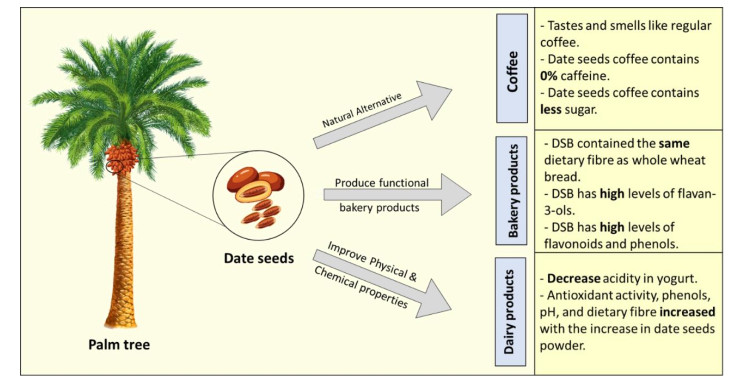
Al-Khalili M, Al-Habsi N, Rahman MS (2023) Applications of date pits in foods to enhance their functionality and quality: A review. Front Sustainable Food Syst 6: 1101043. https://doi.org/10.3389/fsufs.2022.1101043 doi: 10.3389/fsufs.2022.1101043
|
| [77] | Maspul K (2021) Emirati Gahwa Arabiya; a review of signature Arabic coffee in the United Arab Emirates. Academia Letters No.2. https://doi.org/10.20935/AL3655 |
| [78] |
Cornelis MC (2019) The impact of caffeine and coffee on human health. Nutrients 11: 416. https://doi.org/10.3390/nu11020416 doi: 10.3390/nu11020416
|
| [79] |
Venkatachalam CD, Sengottian M (2016) Study on roasted date seed non caffeinated coffee powder as a promising alternative. Asian J Res Soc Sci Humanit 6: 1387. https://doi.org/10.5958/2249-7315.2016.00292.6 doi: 10.5958/2249-7315.2016.00292.6
|
| [80] |
Fikry M, Yusof YA, Al-Awaadh AM, et al. (2019) Effect of the roasting conditions on the physicochemical, quality and sensory attributes of coffee-like powder and brew from defatted palm date seeds. Foods 8: 61. https://doi.org/10.3390/foods8020061 doi: 10.3390/foods8020061
|
| [81] | Abdillah L, Andriani M (2012) Friendly alternative healthy drinks through the use of date seeds as coffee powder. Proceeding of ICEBM 2012: 80–87. |
| [82] |
Ranasinghe M, Manikas I, Maqsood S, et al. (2022) Date components as promising plant-based materials to be incorporated into baked goods—A review. Sustainability 14: 605. https://doi.org/10.3390/su14020605 doi: 10.3390/su14020605
|
| [83] |
Platat C, Habib HM, Hashim IB, et al. (2015) Production of functional pita bread using date seed powder. J Food Sci Technol 52: 6375–6384. https://doi.org/10.1007/s13197-015-1728-0 doi: 10.1007/s13197-015-1728-0
|
| [84] |
Bouaziz F, Abdeddayem A, Koubaa M, et al. (2020) Date seeds as a natural source of dietary fibers to improve texture and sensory properties of wheat bread. Foods 9: 737. https://doi.org/10.3390/foods9060737 doi: 10.3390/foods9060737
|
| [85] |
Najjar Z, Alkaabi M, Alketbi K, et al. (2022) Physical chemical and textural characteristics and sensory evaluation of cookies formulated with date seed powder. Foods 11: 305. https://doi.org/10.3390/foods11030305 doi: 10.3390/foods11030305
|
| [86] |
Abushal SA, Elhendy HA, Maged EM, et al. (2021) Impact of ground Ajwa (Phoenix dactylifera L.) seeds fortification on physical and nutritional properties of functional cookies and chocolate sauce. Cereal Chem 98: 958–967. https://doi.org/10.1002/cche.10437 doi: 10.1002/cche.10437
|
| [87] | Hanan AJ (2018) Evaluation of physio-chemical and sensory properties of yogurt prepared with date pits powder. Curr Sci Int 7: 01–09. |
| [88] |
Darwish AA, Tawfek MA, Baker EA (2020) Texture, sensory attributes and antioxidant activity of spreadable processed cheese with adding date seed powder. J Food Dairy Sci 11: 377–383. https://doi.org/10.21608/jfds.2021.60281.1014 doi: 10.21608/jfds.2021.60281.1014
|
| [89] |
Boeing H, Bechthold A, Bub A, et al. (2012) Critical review: Vegetables and fruit in the prevention of chronic diseases. Eur J Nutr 51: 637–663. https://doi.org/10.1007/s00394-012-0380-y doi: 10.1007/s00394-012-0380-y
|
| [90] | Pem D, Jeewon R (2015) Fruit and vegetable intake: Benefits and progress of nutrition education interventions—Narrative review article. Iran J Public Health 44: 1309–1321. |
| [91] | Brouk M, Fishman A (2016) Antioxidant properties and health benefits of date seeds. In: Kristbergsson K, Ötles S (Eds.), Functional Properties of Traditional Foods, Boston, MA, Springer US, 233–240. https://doi.org/10.1007/978-1-4899-7662-8_16 |
| [92] | Al-Farsi MA, Lee CY (2011) Chapter 53—Usage of date (Phoenix dactylifera L.) seeds in human health and animal feed. In: Preedy VR, Watson RR, Patel VB (Eds.), Nuts and Seeds in Health and Disease Prevention, San Diego, Academic Press, 447–452. https://doi.org/10.1016/B978-0-12-375688-6.10053-2 |
| [93] |
Kharroubi AT, Darwish HM (2015) Diabetes mellitus: The epidemic of the century. World J Diabetes 6: 850–867. https://doi.org/10.4239/wjd.v6.i6.850 doi: 10.4239/wjd.v6.i6.850
|
| [94] | Arshad FK, Jelani DS (2015) A relative in vitro evaluation of antioxidant potential profile of extracts from pits of Phoenix dactylifera L. (Ajwa and Zahedi Dates). Int J Adv Inf Sci Technol 4: 11. |
| [95] |
Saryono S (2019) Date seeds drinking as antidiabetic: A systematic review. IOP Conf Ser: Earth Environ Sci 255: 012018. https://doi.org/10.1088/1755-1315/255/1/012018 doi: 10.1088/1755-1315/255/1/012018
|
| [96] |
Hilary S, Kizhakkayil J, Souka U, et al. (2021) In-vitro investigation of polyphenol-rich date (Phoenix dactylifera L.) seed extract bioactivity. Front Nutr 8: 667514. https://doi.org/10.3389/fnut.2021.667514 doi: 10.3389/fnut.2021.667514
|
| [97] |
Zadeh MM, Dehghan P, Eslami Z (2023) Effect of date seed (Phoenix dactylifera) supplementation as functional food on cardiometabolic risk factors, metabolic endotoxaemia and mental health in patients with type 2 diabetes mellitus: a blinded randomised controlled trial protocol. BMJ Open 13: e066013. https://doi.org/10.1136/bmjopen-2022-066013 doi: 10.1136/bmjopen-2022-066013
|
| [98] |
Khattak MNK, Shanableh A, Hussain MI, et al. (2020) Anticancer activities of selected Emirati Date (Phoenix dactylifera L.) varieties pits in human triple negative breast cancer MDA-MB-231 cells. Saudi J Biol Sci 27: 3390–3396. https://doi.org/10.1016/j.sjbs.2020.09.001 doi: 10.1016/j.sjbs.2020.09.001
|
| [99] |
Rezaei M, Khodaei F, Hooshmand N (2015) Date seed extract diminished apoptosis event in human colorectal carcinoma cell line. MOJ Toxicol 1: 00017. https://doi.org/10.15406/mojt.2015.01.00017 doi: 10.15406/mojt.2015.01.00017
|
| [100] |
Sia J, Szmyd R, Hau E, et al. (2020) Molecular mechanisms of radiation-induced cancer cell death: A primer. Front Cell Dev Biol 8: 41. https://doi.org/10.3389/fcell.2020.00041 doi: 10.3389/fcell.2020.00041
|
| [101] |
Khezerloo D, Mortezazadeh T, Farhood B, et al. (2019) The effect of date palm seed extract as a new potential radioprotector in gamma-irradiated mice. J Cancer Res Ther 15: 517. https://doi.org/10.4103/jcrt.JCRT_1341_16 doi: 10.4103/jcrt.JCRT_1341_16
|
| [102] |
Juhaimi FA, Ghafoor K, Özcan MM (2012) Physical and chemical properties, antioxidant activity, total phenol and mineral profile of seeds of seven different date fruit (Phoenix dactylifera L.) varieties. Int J Food Sci Nutr 63: 84–89. https://doi.org/10.3109/09637486.2011.598851 doi: 10.3109/09637486.2011.598851
|
| [103] |
Olaniyi OO, Samuel IA, Igbe FO (2022) Phytochemical content, antioxidant properties and antibacterial activities of date (Phoenix dactylifera L.) seed extracts. J Food Saf Hyg 8: 78–93. https://doi.org/10.18502/jfsh.v8i2.10670 doi: 10.18502/jfsh.v8i2.10670
|
| [104] |
Alrajhi M, AL-Rasheedi M, Eltom SEM, et al. (2019) Antibacterial activity of date palm cake extracts (Phoenix dactylifera). Cogent Food Agric 5: 1625479. https://doi.org/10.1080/23311932.2019.1625479 doi: 10.1080/23311932.2019.1625479
|
| [105] |
Selim S, Abdel-Mawgoud M, Al-sharary T, et al. (2022) Pits of date palm: Bioactive composition, antibacterial activity and antimutagenicity potentials. Agronomy 12: 54. https://doi.org/10.3390/agronomy12010054 doi: 10.3390/agronomy12010054
|
| [106] |
Saddiq AA, Bawazir AE (2010) Antimicrobial activity of date palm (Phoenix dactylifera) pits extracts and its role in reducing side effect of methyl prednisolone on some neurotransmitter content in the brain, hormone testosterone in adulthood. ISHS Acta Hortic 882: 665–690. https://doi.org/10.17660/ActaHortic.2010.882.74 doi: 10.17660/ActaHortic.2010.882.74
|
| [107] |
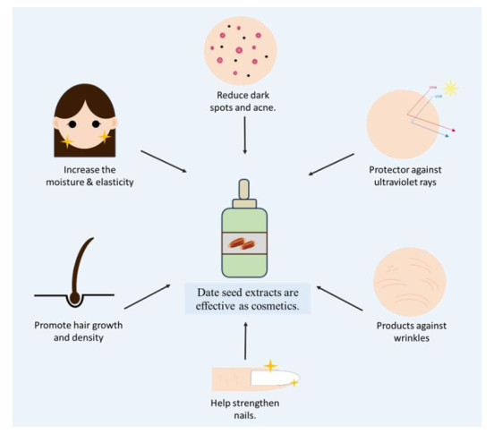
Alharbi KL, Raman J, Shin HJ (2021) Date fruit and seed in nutricosmetics. Cosmetics 8: 59. https://doi.org/10.3390/cosmetics8030059 doi: 10.3390/cosmetics8030059
|
| [108] |
Cherubim DJ, Martins CV, Fariña L, et al. (2020) Polyphenols as natural antioxidants in cosmetics applications. J Cosmet Dermatol 19: 33–37. https://doi.org/10.1111/jocd.13093 doi: 10.1111/jocd.13093
|
| [109] |
Patel S, Sharma V, Chauhan NS, et al. (2015) Hair growth: Focus on herbal therapeutic agent. Curr Drug Discovery Technol 12: 21–42. https://doi.org/10.2174/1570163812666150610115055 doi: 10.2174/1570163812666150610115055
|
| [110] |
Hong YJ, Tomas-Barberan FA, Kader AA, et al. (2006) The flavonoid glycosides and procyanidin composition of Deglet Noor Dates (Phoenix dactylifera). J Agric Food Chem 54: 2405–2411. https://doi.org/10.1021/jf0581776 doi: 10.1021/jf0581776
|
| [111] |
Dattola A, Silvestri M, Bennardo L, et al. (2020) Role of vitamins in skin health: A systematic review. Curr Nutr Rep 9: 226–235. https://doi.org/10.1007/s13668-020-00322-4 doi: 10.1007/s13668-020-00322-4
|
| [112] | Mohammadi M, Soltani M, Siahpoosh A, et al. (2018) Effects of dietary supplementation of date palm (Phoenix dactylifera) seed extract on body composition, lipid peroxidation and tissue quality of common carp (Cyprinus carpio) juveniles based on the total volatile nitrogen test. Iran J Fish Sci 17: 394–402. |
| [113] |
Arshad N, Samat N, Lee LK (2022) Insight into the relation between nutritional benefits of aquaculture products and its consumption hazards: A global viewpoint. Front Mar Sci 9: 925463. https://doi.org/10.3389/fmars.2022.925463 doi: 10.3389/fmars.2022.925463
|
| [114] |
Metian M, Troell M, Christensen V, et al. (2020) Mapping diversity of species in global aquaculture. Rev Aquacult 12: 1090–1100. https://doi.org/10.1111/raq.12374 doi: 10.1111/raq.12374
|
| [115] |
Naylor RL, Hardy RW, Buschmann AH, et al. (2021) A 20-year retrospective review of global aquaculture. Nature 591: 551–563. https://doi.org/10.1038/s41586-021-03308-6 doi: 10.1038/s41586-021-03308-6
|
| [116] | Software for Fishery and Aquaculture Statistical Time Series Food and Agriculture Organization of the United Nations FAO. Available from: https://www.fao.org/fishery/en/topic/166235/en. |
| [117] |
Sotolu A, Kigbu A, Oshinowo A (2014) Supplementation of date palm (Phoenix dactylifera) seed as feed additive in the diets of juvenile African catfish (Burchell, 1822). J Fish Aquat Sci 9: 359–365. https://doi.org/10.3923/jfas.2014.359.365 doi: 10.3923/jfas.2014.359.365
|
| [118] |
Hua K, Cobcroft JM, Cole A, et al. (2019) The future of aquatic protein: Implications for protein sources in aquaculture diets. One Earth 1: 316–329. https://doi.org/10.1016/j.oneear.2019.10.018 doi: 10.1016/j.oneear.2019.10.018
|
| [119] | García-Beltrán JM, Mahdhi A, Abdelkader N, et al. (2020) Effect of the administration of date palm seeds (Phoenix dactylifera L.) in Gilthead Seabream (Sparus aurata L.) Diets. 1: 21. |
| [120] |
Mohammadi M, Soltani M, Siahpoosh A, et al. (2018) Effect of date palm (Phoenix dactylifera) seed extract as a dietary supplementation on growth performance immunological haematological biochemical parameters of common carp. Aquacult Res 49: 2903–2912. https://doi.org/10.1111/are.13760 doi: 10.1111/are.13760
|
| [121] |
Dawood MAO, Eweedah NM, Khalafalla MM, et al. (2020) Evaluation of fermented date palm seed meal with Aspergillus oryzae on the growth, digestion capacity and immune response of Nile tilapia (Oreochromis niloticus). Aquacult Nutr 26: 828–841. https://doi.org/10.1111/anu.13042 doi: 10.1111/anu.13042
|
| [122] | FAO: Common carp home Food and Agriculture Organization of the United Nations FAO. Available from: https://www.fao.org/fishery/affris/species-profiles/common-carp/common-carp-home/en/. |
| [123] | Prospecting the biofuel potential of the UAE's 'Allig' date seed issuu. Available from: https://issuu.com/moeuae/docs/explorer_6456_research_magazine_edition_2_en_final/s/11762721. |
| [124] |
Cruz-Lovera C, Manzano-Agugliaro F, Salmerón-Manzano E, et al. (2019) Date seeds (Phoenix dactylifera L.) valorization for boilers in the Mediterranean climate. Sustainability 11: 711. https://doi.org/10.3390/su11030711 doi: 10.3390/su11030711
|
| [125] |
Mousa R (2016) Hydrocolloids of date pits used as edible coating to reduce oil uptake in potato strips during deep-fat frying. Alexandria J Food Sci Technol 13: 39–50. https://doi.org/10.12816/0038469 doi: 10.12816/0038469
|
Figures(4) / Tables(3)

Asma Hussain Alkatheri, Mahra Saleh Alkatheeri, Wan-Hee Cheng, Warren Thomas, Kok-Song Lai, Swee-Hua Erin Lim. Innovations in extractable compounds from date seeds: Farms to future[J]. AIMS Agriculture and Food, 2024, 9(1): 256-281. doi: 10.3934/agrfood.2024016


 DownLoad: