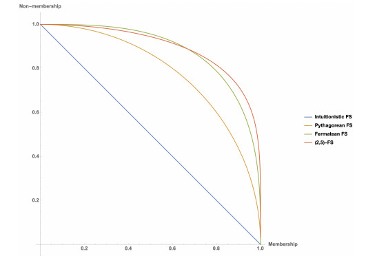
Many models of uncertain knowledge have been designed that combine expanded views of fuzziness (expressions of partial memberships) with parameterization (multiple subsethood indexed by a parameter set). The standard orthopair fuzzy soft set is a very general example of this successful blend initiated by fuzzy soft sets. It is a mapping from a set of parameters to the family of all orthopair fuzzy sets (which allow for a very general view of acceptable membership and non-membership evaluations). To expand the scope of application of fuzzy soft set theory, the restriction of orthopair fuzzy sets that membership and non-membership must be calibrated with the same power should be removed. To this purpose we introduce the concept of $ (a, b) $-fuzzy soft set, shortened as $ (a, b) $-FSS. They enable us to address situations that impose evaluations with different importances for membership and non-membership degrees, a problem that cannot be modeled by the existing generalizations of intuitionistic fuzzy soft sets. We establish the fundamental set of arithmetic operations for $ (a, b) $-FSSs and explore their main characteristics. Then we define aggregation operators for $ (a, b) $-FSSs and discuss their main properties and the relationships between them. Finally, with the help of suitably defined scores and accuracies we design a multi-criteria decision-making strategy that operates in this novel framework. We also analyze a decision-making problem to endorse the validity of $ (a, b) $-FSSs for decision-making purposes.
Citation: Tareq M. Al-shami, José Carlos R. Alcantud, Abdelwaheb Mhemdi. New generalization of fuzzy soft sets: $ (a, b) $-Fuzzy soft sets[J]. AIMS Mathematics, 2023, 8(2): 2995-3025. doi: 10.3934/math.2023155
Many models of uncertain knowledge have been designed that combine expanded views of fuzziness (expressions of partial memberships) with parameterization (multiple subsethood indexed by a parameter set). The standard orthopair fuzzy soft set is a very general example of this successful blend initiated by fuzzy soft sets. It is a mapping from a set of parameters to the family of all orthopair fuzzy sets (which allow for a very general view of acceptable membership and non-membership evaluations). To expand the scope of application of fuzzy soft set theory, the restriction of orthopair fuzzy sets that membership and non-membership must be calibrated with the same power should be removed. To this purpose we introduce the concept of $ (a, b) $-fuzzy soft set, shortened as $ (a, b) $-FSS. They enable us to address situations that impose evaluations with different importances for membership and non-membership degrees, a problem that cannot be modeled by the existing generalizations of intuitionistic fuzzy soft sets. We establish the fundamental set of arithmetic operations for $ (a, b) $-FSSs and explore their main characteristics. Then we define aggregation operators for $ (a, b) $-FSSs and discuss their main properties and the relationships between them. Finally, with the help of suitably defined scores and accuracies we design a multi-criteria decision-making strategy that operates in this novel framework. We also analyze a decision-making problem to endorse the validity of $ (a, b) $-FSSs for decision-making purposes.

| [1] |
B. Ahmad, A. Kharal, On fuzzy soft sets, Adv. Fuzzy Syst., 2009 (2009). https://doi.org/10.1155/2009/586507 doi: 10.1155/2009/586507

|
| [2] |
M. Akram, A. Adeel, J. C. R. Alcantud, Fuzzy $N$-soft sets: A novel model with applications, J. Intell. Fuzzy Syst., 35 (2018), 4757–4771. https://doi.org/10.3233/JIFS-18244 doi: 10.3233/JIFS-18244
|
| [3] |
J. C. R. Alcantud, Convex soft geometries, J. Comput. Cognitive Eng., 1 (2022), 2–12. https://doi.org/10.47852/bonviewJCCE597820 doi: 10.47852/bonviewJCCE597820
|
| [4] |
J. C. R. Alcantud, The semantics of $N$-soft sets, their applications, and a coda about three-way decision, Inform. Sci., 606 (2022), 837–852. https://doi.org/10.1016/j.ins.2022.05.084 doi: 10.1016/j.ins.2022.05.084
|
| [5] |
J. C. R. Alcantud, T. M. Al-shami, A. A. Azzam, Caliber and chain conditions in soft topologies, Mathematics, 9 (2021), 2349. https://doi.org/10.3390/math9192349 doi: 10.3390/math9192349
|
| [6] |
J. C. R. Alcantud, A. Z. Khameneh, A. Kilicman, Aggregation of infinite chains of intuitionistic fuzzy sets and their application to choices with temporal intuitionistic fuzzy information, Inform. Sci., 514 (2020), 106–117. https://doi.org/10.1016/j.ins.2019.12.008 doi: 10.1016/j.ins.2019.12.008
|
| [7] |
J. C. R. Alcantud, G. Varela, B. Santos-Buitrago, G. Santos-García, M. F. Jiménez, Analysis of survival for lung cancer resections cases with fuzzy and soft set theory in surgical decision making, Plos One, 14 (2019), e0218283. https://doi.org/10.1371/journal.pone.0218283 doi: 10.1371/journal.pone.0218283
|
| [8] |
T. M. Al-shami, (2, 1)-Fuzzy sets: Properties, weighted aggregated operators and their applications to multi-criteria decision-making methods, Complex Intell. Syst., 2022. https://doi.org/10.1007/s40747-022-00878-4 doi: 10.1007/s40747-022-00878-4
|
| [9] | T. M. Al-shami, Generalized umbral for orthopair fuzzy sets: (m, n)-Fuzzy sets and their applications to multi-criteria decision-making methods, Submitted. |
| [10] |
T. M. Al-shami, Soft somewhat open sets: Soft separation axioms and medical application to nutrition, Comput. Appl. Math., 41 (2022), 216. https://doi.org/10.1007/s40314-022-01919-x doi: 10.1007/s40314-022-01919-x
|
| [11] |
T. M. Al-shami, H. Z. Ibrahim, A. A. Azzam, A. I. EL-Maghrabi, SR-fuzzy sets and their applications to weighted aggregated operators in decision-making, J. Funct. Space., 2022 (2022). https://doi.org/10.1155/2022/3653225 doi: 10.1155/2022/3653225
|
| [12] |
T. M. Al-shami, L. D. R. Kočinac, Almost soft Menger and weakly soft Menger spaces, Appl. Comput. Math., 21 (2022), 35–51. https://doi.org/10.30546/1683-6154.21.1.2022.35 doi: 10.30546/1683-6154.21.1.2022.35
|
| [13] |
T. M. Al-shami, A. Mhemdi, R. Abu-Gdairi, M. E. El-Shafei, Compactness and connectedness via the class of soft somewhat open sets, AIMS Math., 8 (2023), 815–840. https://doi.org/10.3934/math.2023040 doi: 10.3934/math.2023040
|
| [14] |
T. M. Al-shami, A. Mhemdi, A. Rawshdeh, H. Al-jarrah, Soft version of compact and Lindelöf spaces using soft somewhere dense set, AIMS Math., 6 (2021), 8064–8077. https://doi.org/10.3934/math.2021468 doi: 10.3934/math.2021468
|
| [15] |
Z. A. Ameen, T. M. Al-shami, A. A. Azzam, A. Mhemdi, A novel fuzzy structure: Infra-fuzzy topological spaces, J. Funct. Space., 2022 (2022) https://doi.org/10.1155/2022/9778069 doi: 10.1155/2022/9778069
|
| [16] | K. T. Atanassov, Intuitionistic fuzzy sets, Fuzzy Set. Syst., 20 (1986), 87–96. |
| [17] |
M. Atef, M. I. Ali, T. M. Al-shami, Fuzzy soft covering-based multi-granulation fuzzy rough sets and their applications, Comput. Appl. Math., 40 (2021), 115. https://doi.org/10.1007/s40314-021-01501-x doi: 10.1007/s40314-021-01501-x
|
| [18] | N. Cağman, S. Enginoğlu, F. Çitak, Fuzzy soft set theory and its application, Iran. J. Fuzzy Syst., 8 (2011), 137–147. |
| [19] |
S. K. De, R. B. Akhil, R. Roy, An application of intuitionistic fuzzy sets in medical diagnosis, Fuzzy Set. Syst., 117 (2001), 209–213. https://doi.org/10.1016/S0165-0114(98)00235-8 doi: 10.1016/S0165-0114(98)00235-8
|
| [20] |
F. Fatimah, D. Rosadi, R. B. F. Hakim, J. C. R. Alcantud, $N$-soft sets and their decision-making algorithms, Soft Comput., 22 (2018), 3829–3842. https://doi.org/10.1007/s00500-017-2838-6 doi: 10.1007/s00500-017-2838-6
|
| [21] |
F. Fatimah, J. C. R. Alcantud, The multi-fuzzy $N$-soft set and its applications to decision-making, Neural Comput. Appl., 33 (2021), 11437–11446. https://doi.org/10.1007/s00521-020-05647-3 doi: 10.1007/s00521-020-05647-3
|
| [22] |
M. Gulzar, D. Alghazzawi, M. H. Mateen, N. Kausar, A certain class of t-intuitionistic fuzzy subgroups, IEEE Access, 8 (2020), 163260–163268. https://doi.org/10.1109/ACCESS.2020.3020366 doi: 10.1109/ACCESS.2020.3020366
|
| [23] |
M. T. Hamida, M. Riaz, D. Afzal, Novel MCGDM with q-rung orthopair fuzzy soft sets and TOPSIS approach under q-Rung orthopair fuzzy soft topology, J. Intell. Fuzzy Syst., 39 (2020), 3853–3871. https://doi.org/10.3233/JIFS-192195 doi: 10.3233/JIFS-192195
|
| [24] |
H. Z. Ibrahim, T. M. Al-shami, O. G. Elbarbary, (3, 2)-Fuzzy sets and their applications to topology and optimal choices, Comput. Intell. Neurosci., 2021 (2021). https://doi.org/10.1155/2021/1272266 doi: 10.1155/2021/1272266
|
| [25] | S. J. John, Soft sets: Theory and applications, Springer Cham, 2021. |
| [26] |
H. Liao, Z. Xu, Intuitionistic fuzzy hybrid weighted aggregation operators, Int. J. Intell. Syst., 29 (2014), 971–993. https://doi.org/10.1002/int.21672 doi: 10.1002/int.21672
|
| [27] |
A. A. Khan, S. Ashraf, S. Abdullah, M. Qiyas, J. Luo, S. U. Khan, Pythagorean fuzzy Dombi aggregation operators and their application in decision support system, Symmetry, 11 (2019), 383. https://doi.org/10.3390/sym11030383 doi: 10.3390/sym11030383
|
| [28] | M. Kirişci, A case study for medical decision making with the fuzzy soft sets, Afr. Mat., 31 (2020), 557–564. |
| [29] |
M. Kirişci, N. Şimşek, Decision making method related to Pythagorean fuzzy soft sets with infectious diseases application, J. King Saud Univ.-Com., 34 (2022), 5968–5978. https://doi.org/10.1016/j.jksuci.2021.08.010 doi: 10.1016/j.jksuci.2021.08.010
|
| [30] | P. K. Maji, R. Biswas, A. R. Roy, Fuzzy soft sets, J. Fuzzy Math., 9 (2001), 589–602. |
| [31] |
A. R. Roy, P. K. Maji, A fuzzy soft set theoretic approach to decision making problems, J. Comput. Appl. Math., 203 (2007), 412–418. https://doi.org/10.1016/j.cam.2006.04.008 doi: 10.1016/j.cam.2006.04.008
|
| [32] |
D. Molodtsov, Soft set theory–-first results, Comput. Math. Appl., 37 (1999), 19–31. https://doi.org/10.1016/S0898-1221(99)00056-5 doi: 10.1016/S0898-1221(99)00056-5
|
| [33] |
X. Peng, H. Yuan, Fundamental properties of Pythagorean fuzzy aggregation operators, Fund. Inform., 147 (2016), 415–446. https://doi.org/10.3233/FI-2016-1415 doi: 10.3233/FI-2016-1415
|
| [34] | X. Peng, Y. Yang, J. Song, Y. Jiang, Pythagorean fuzzy soft set and its application, Comput. Eng., 41 (2015), 224–229. |
| [35] |
K. Rahman, S. Abdullah, M. Jamil, M. Y. Khan, Some generalized intuitionistic fuzzy Einstein hybrid aggregation operators and their application to multiple attribute group decision making, Int. J. Fuzzy Syst., 20 (2018), 1567–1575. https://doi.org/10.1007/s40815-018-0452-0 doi: 10.1007/s40815-018-0452-0
|
| [36] | K. Rahman, S. Abdullah, M. S. A. Khan, M. Shakeel, Pythagorean fuzzy hybrid geometric aggregation operator and their applications to multiple attribute decision making, Int. J. Comput. Sci. Inform. Sec., 14 (2016), 837–854. |
| [37] | A. Sivadas, S. J. John, Fermatean fuzzy soft sets and its applications, Communications in Computer and Information Science, Springer, Singapore, 1345 (2021). |
| [38] |
S. Saleh, R. Abu-Gdairi, T. M. Al-shami, Mohammed S. Abdo, On categorical property of fuzzy soft topological spaces, Appl. Math. Inform. Sci., 16 (2022), 635–641. http://dx.doi.org/10.18576/amis/160417 doi: 10.18576/amis/160417
|
| [39] |
T. Senapati, R. R. Yager, Fermatean fuzzy weighted averaging/geometric operators and its application in multi-criteria decision-making methods, Eng. Appl. Artif. Intell., 85 (2019), 112–121. https://doi.org/10.1016/j.engappai.2019.05.012 doi: 10.1016/j.engappai.2019.05.012
|
| [40] |
T. Senapati, R. R. Yager, Fermatean fuzzy sets, J. Amb. Intell. Hum. Comput., 11 (2020), 663–674. https://doi.org/10.1007/s12652-019-01377-0 doi: 10.1007/s12652-019-01377-0
|
| [41] | Y. J. Xu, Y. K. Sun, D. F. Li, Intuitionistic fuzzy soft set, 2010 2nd International Workshop on Intelligent Systems and Applications, 2010, 1–4. https://doi.org/10.1109/IWISA.2010.5473444 |
| [42] |
J. Wan, H. Chen, T. Li, Z. Yuan, J. Liu, W. Huang, Interactive and complementary feature selection via fuzzy multigranularity uncertainty measures, IEEE T. Cybern., 2021. https://doi.org/10.1109/TCYB.2021.3112203 doi: 10.1109/TCYB.2021.3112203
|
| [43] |
R. R. Yager, Pythagorean membership grades in multicriteria decision making, IEEE T. Fuzzy Syst., 22 (2013), 958–965. https://doi.org/10.1109/TFUZZ.2013.2278989 doi: 10.1109/TFUZZ.2013.2278989
|
| [44] |
R. R. Yager, Generalized orthopair fuzzy sets, IEEE T. Fuzzy Syst., 25 (2017), 1222–1230. https://doi.org/10.1109/TFUZZ.2016.2604005 doi: 10.1109/TFUZZ.2016.2604005
|
| [45] |
B. Yang, Fuzzy covering-based rough set on two different universes and its application, Artif. Intell. Rev., 55 (2022), 4717–4753. https://doi.org/10.1007/s10462-021-10115-y doi: 10.1007/s10462-021-10115-y
|
| [46] |
B. Yang, B. Q. Hu, A fuzzy covering-based rough set model and its generalization over fuzzy lattice, Inform. Sci., 367–368 (2016), 463–486. https://doi.org/10.1016/j.ins.2016.05.053 doi: 10.1016/j.ins.2016.05.053
|
| [47] |
J. Yang, Y. Yao, Semantics of soft sets and three-way decision with soft sets, Inform. Sci., 194 (2020), 105538. https://doi.org/10.1016/j.knosys.2020.105538 doi: 10.1016/j.knosys.2020.105538
|
| [48] | L. A. Zadeh, Fuzzy sets, Inform. Control, 8 (1965), 338–353. |

Figures(2) / Tables(5)

Tareq M. Al-shami, José Carlos R. Alcantud, Abdelwaheb Mhemdi. New generalization of fuzzy soft sets: $ (a, b) $-Fuzzy soft sets[J]. AIMS Mathematics, 2023, 8(2): 2995-3025. doi: 10.3934/math.2023155


 DownLoad: