Optimization and evaluation of resveratrol amorphous solid dispersions with a novel polymeric system

Gangqi Han; Bing Wang; Mengli Jia; Shuxin Ding; Wenxuan Qiu; Yuxuan Mi; Zhimei Mi; Yuhao Qin; Wenxing Zhu; Xinli Liu; Wei Li; Gangqi Han; Bing Wang; Mengli Jia; Shuxin Ding; Wenxuan Qiu; Yuxuan Mi; Zhimei Mi; Yuhao Qin; Wenxing Zhu; Xinli Liu; Wei Li

doi:10.3934/mbe.2022375

Mathematical Biosciences and Engineering

2022, Volume 19, Issue 8: 8019-8034. doi: 10.3934/mbe.2022375

Previous Article Next Article

Research article

Optimization and evaluation of resveratrol amorphous solid dispersions with a novel polymeric system

1.
State Key Laboratory of Bio-based Material and Green Papermaking (LBMP), Qilu University of Technology (Shandong Academy of Sciences), Jinan, Shandong, China
2.
Key Laboratory of Shandong Microbial Engineering, School of Bioengineering, Qilu University of Technology (Shandong Academy of Sciences), Jinan, Shandong, China
3.
College of Pharmacy, Heze University, Heze, Shandong, China
4.
Shandong Dashu Dafute Food Co., Ltd, Heze, Shandong, China
5.
Shandong Medical College, Jinan, Shandong, China

† These two authors are designated as the co-first authors who made equal contributions to this study.
Academic Editor: Chiara Giulia Fontanella

Received: 01 March 2022 Revised: 10 April 2022 Accepted: 22 April 2022 Published: 31 May 2022

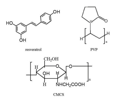
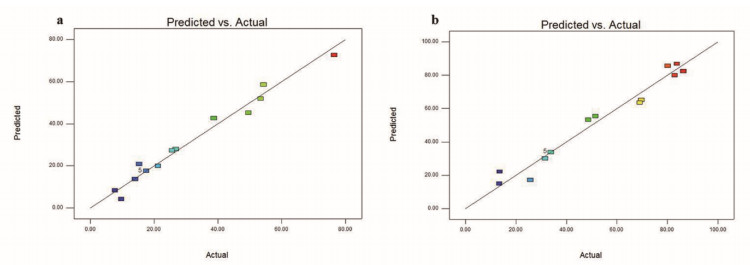
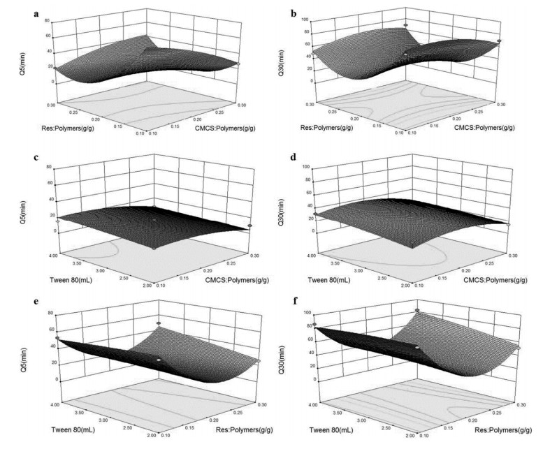
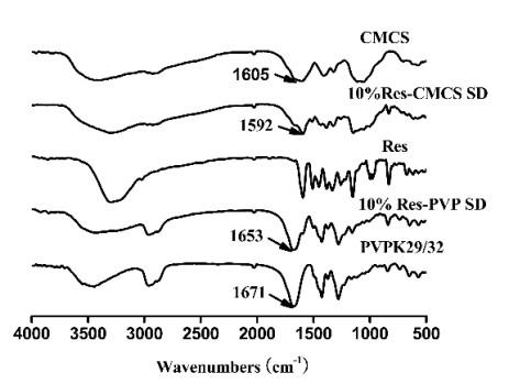
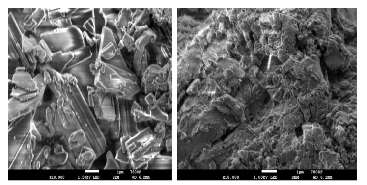
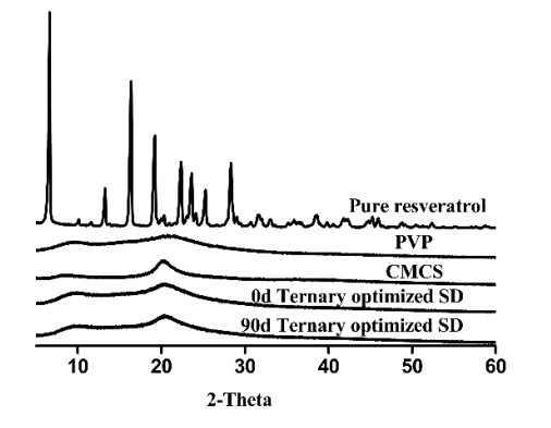
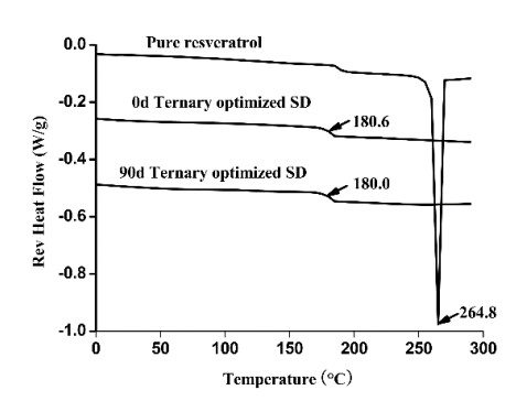
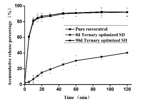
The preparation of amorphous solid dispersions using polymers is a commonly used formulation strategy for enhancing the solubility of poorly water-soluble drugs. However, a single polymer often does not bring significantly enhance the solubility or amorphous stability of a poorly water-soluble drug. We found an application of a unique and novel binary polymeric blend in the preparation of solid dispersions. The main purpose of this study is to optimize and evaluate resveratrol (Res) amorphous solid dispersions with a novel polymeric system of poly (vinyl pyrrolidone) (PVP) and carboxymethyl chitosan (CMCS). The influence of three different release factors, the ratio of CMCS to the polymer mixture (CMCS% = X₁), the ratio of Res to the polymer mixture (Res% = X₂) and the surfactant (Tween 80 = X₃), on the characteristics of released Res at various times (Q₅ and Q₃₀) was investigated. The computer optimization and contour plots were used to predict the levels of the independent variables as X₁ = 0.17, X₂ = 0.10 and X₃ = 2.94 for maximized responses of Q₅ and Q₃₀. Fourier transform infrared spectroscopy (FTIR) results revealed that each polymer formed hydrogen bonds with Res. The solid performance and physical stability of the optimized ternary dispersions were studied with scanning electron microscopy (SEM), powder X-ray diffraction (XRD), modulated differential scanning calorimetry (MDSC) and dissolution testing. SEM, XRD and MDSC analysis demonstrated that the Res was amorphous, and MDSC showed no evidence of phase separation during storage. Dissolution testing indicated a more than fourfold increase in the apparent solubility of the optimized ternary dispersions, which maintained high solubility after 90 days. In our research, we used CMCS as a new carrier in combination with PVP, which not only improved the in vitro dissolution of Res but also had better stability.
- resveratrol,
- solid dispersions,
- PVP,
- CMCS,
- Box–Behnken design,
- stability
Citation: Gangqi Han, Bing Wang, Mengli Jia, Shuxin Ding, Wenxuan Qiu, Yuxuan Mi, Zhimei Mi, Yuhao Qin, Wenxing Zhu, Xinli Liu, Wei Li. Optimization and evaluation of resveratrol amorphous solid dispersions with a novel polymeric system[J]. Mathematical Biosciences and Engineering, 2022, 19(8): 8019-8034. doi: 10.3934/mbe.2022375

Related Papers:

Abstract

The preparation of amorphous solid dispersions using polymers is a commonly used formulation strategy for enhancing the solubility of poorly water-soluble drugs. However, a single polymer often does not bring significantly enhance the solubility or amorphous stability of a poorly water-soluble drug. We found an application of a unique and novel binary polymeric blend in the preparation of solid dispersions. The main purpose of this study is to optimize and evaluate resveratrol (Res) amorphous solid dispersions with a novel polymeric system of poly (vinyl pyrrolidone) (PVP) and carboxymethyl chitosan (CMCS). The influence of three different release factors, the ratio of CMCS to the polymer mixture (CMCS% = X₁), the ratio of Res to the polymer mixture (Res% = X₂) and the surfactant (Tween 80 = X₃), on the characteristics of released Res at various times (Q₅ and Q₃₀) was investigated. The computer optimization and contour plots were used to predict the levels of the independent variables as X₁ = 0.17, X₂ = 0.10 and X₃ = 2.94 for maximized responses of Q₅ and Q₃₀. Fourier transform infrared spectroscopy (FTIR) results revealed that each polymer formed hydrogen bonds with Res. The solid performance and physical stability of the optimized ternary dispersions were studied with scanning electron microscopy (SEM), powder X-ray diffraction (XRD), modulated differential scanning calorimetry (MDSC) and dissolution testing. SEM, XRD and MDSC analysis demonstrated that the Res was amorphous, and MDSC showed no evidence of phase separation during storage. Dissolution testing indicated a more than fourfold increase in the apparent solubility of the optimized ternary dispersions, which maintained high solubility after 90 days. In our research, we used CMCS as a new carrier in combination with PVP, which not only improved the in vitro dissolution of Res but also had better stability.

References

[1]	S. Rani, R. Rana, G. K. Saraogi, V. Kumar, U. Gupta, Self-emulsifying oral lipid drug delivery systems: Advances and challenges, AAPS PharmSciTech, 20 (2019), 2–12. https://doi.org/10.1208/s12249-019-1335-x doi: 10.1208/s12249-019-1335-x
[2]	G. Amidon, H. Lennernäs, V. Shah, J. Crison, A theoretical basis for a biopharmaceutic drug classification: The correlation of in vitro drug product dissolution and in vivo bioavailability, Pharm. Res., 12 (1995), 413–420. https://doi.org/10.1023/A:1016212804288 doi: 10.1023/A:1016212804288
[3]	S. Feng, Y. Yang, Z. Yang, Z. Wang, L. Yan, F. Wang, et al., Hyaluronic acid-endostatin2-alft1 (ha-es2-af) nanoparticle-like conjugate for the target treatment of diseases, J. Controlled Release, 288 (2018), 1–13. https://doi.org/10.1016/j.jconrel.2018.08.038 doi: 10.1016/j.jconrel.2018.08.038
[4]	S. Watano, M. Matsuo, H. Nakamura, T. Miyazaki, Improvement of dissolution rate of poorly water-soluble drug by wet grinding with bio-compatible phospholipid polymer, Chem. Eng. Sci., 125 (2015), 25–31. https://doi.org/10.1016/j.ces.2014.09.010 doi: 10.1016/j.ces.2014.09.010
[5]	S. A. Zolotov, N. B. Demina, A. S. Zolotova, N. V. Shevlyagina, G. A. Buzanov, V. M. Retivov, et al., Development of novel darunavir amorphous solid dispersions with mesoporous carriers, Eur. J. Pharm. Sci., 159 (2021), 105700. https://doi.org/10.1016/j.ejps.2021.105700 doi: 10.1016/j.ejps.2021.105700
[6]	K. Y. Nam, S. M. Cho, Y. W. Choi, C. Park, N. M. Meghani, J. B. Park, et al., Double controlled release of highly insoluble cilostazol using surfactant-driven ph dependent and ph-independent polymeric blends and in vivo bioavailability in beagle dogs, Int. J. Pharm., 558 (2019), 284–290. https://doi.org/10.1016/j.ijpharm.2019.01.004 doi: 10.1016/j.ijpharm.2019.01.004
[7]	N. Li, N. Wang, T. Wu, C. Qiu, X. Wang, S. Jiang, et al., Preparation of curcumin-hydroxypropyl-β-cyclodextrin inclusion complex by cosolvency-lyophilization procedure to enhance oral bioavailability of the drug, Drug Dev. Ind. Pharm., 44 (2018), 1966–1974. https://doi.org/10.1080/03639045.2018.1505904 doi: 10.1080/03639045.2018.1505904
[8]	J. Li, I. W. Lee, G. H. Shin, X. Chen, H. J. Park, Curcumin-Eudragit® E PO solid dispersion: A simple and potent method to solve the problems of curcumin, Eur. J. Pharm. Biopharm., 94 (2015), 322–332. https://doi.org/10.1016/j.ejpb.2015.06.002 doi: 10.1016/j.ejpb.2015.06.002
[9]	M. Shergill, M. Patel, S. Khan, A. Bashir, C. Mcconville, Development and characterisation of sustained release solid dispersion oral tablets containing the poorly water soluble drug disulfiram, Int. J. Pharm., 497 (2015), 3–11. https://doi.org/10.1016/j.ijpharm.2015.11.029 doi: 10.1016/j.ijpharm.2015.11.029
[10]	J. F. Savouret, M. Quesne, Resveratrol and cancer: A review, Biomed. Pharmacother., 56 (2002), 84–87. https://doi.org/10.1016/S0753-3322(01)00158-5 doi: 10.1016/S0753-3322(01)00158-5
[11]	J. Sharifi-Rad, C. Quispe, A. Durazzo, M. Lucarini, E. B. Souto, A. Santini, et al., Resveratrol' biotechnological applications: Enlightening its antimicrobial and antioxidant properties, J. Herb. Med., 32 (2022), 100550. https://doi.org/10.1016/j.hermed.2022.100550 doi: 10.1016/j.hermed.2022.100550
[12]	A. Alesci, N. Nicosia, A. Fumia, F. Giorgianni, A. Santini, N. Cicero, Resveratrol and immune cells: A link to improve human health, Molecules, 27 (2022), 424. https://doi.org/10.3390/molecules27020424 doi: 10.3390/molecules27020424
[13]	R. B. Rigon, N. Fachinetti, P. Severino, A. Durazzo, M. Lucarini, A. G. Atanasov, et al., Quantification of trans-resveratrol-loaded solid lipid nanoparticles by a validated reverse-phase HPLC photodiode array, Appl. Sci., 9 (2019), 4961. https://doi.org/10.3390/app9224961 doi: 10.3390/app9224961
[14]	A. C. Santos, F. Veiga, A. J. Ribeiro, New delivery systems to improve the bioavailability of resveratrol, Expert Opin. Drug Delivery, 8 (2011), 973–990. https://doi.org/10.1517/17425247.2011.581655 doi: 10.1517/17425247.2011.581655
[15]	A. Amri, J. C. Chaumeil, S. Sfar, C. Charrueau, Administration of resveratrol: What formulation solutions to bioavailability limitations, J. Controlled Release, 158 (2012), 182–193. https://doi.org/10.1016/j.jconrel.2011.09.083 doi: 10.1016/j.jconrel.2011.09.083
[16]	J. S. Sohn, J. S. Kim, J. S. Choi, Development of a naftopidil-chitosan-based fumaric acid solid dispersion to improve the dissolution rate and stability of naftopidil, Int. J. Biol. Macromol., 176 (2021), 520–529. https://doi.org/10.1016/j.ijbiomac.2021.02.096 doi: 10.1016/j.ijbiomac.2021.02.096
[17]	T. Vasconcelos, F. Prezotti, F. Araújo, C. Lopes, A. Loureiro, S. Marques, et al., Third-generation solid dispersion combining Soluplus and poloxamer 407 enhances the oral bioavailability of resveratrol, Int. J. Pharm., 595 (2021), 120245. https://doi.org/10.1016/j.ijpharm.2021.120245 doi: 10.1016/j.ijpharm.2021.120245
[18]	B. Li, L. A. Wegiel, L. S. Taylor, K. J. Edgar, Stability and solution concentration enhancement of resveratrol by solid dispersion in cellulose derivative matrices, Cellulose, 20 (2013), 1249–1260. https://doi.org/10.1007/s10570-013-9889-3 doi: 10.1007/s10570-013-9889-3
[19]	T. Andreani, J. S. Fangueiro, S. José, A. Santini, A. M. Silva, E. B. Souto, Hydrophilic polymers for modified-release nanoparticles: A review of mathematical modelling for pharmacokinetic analysis, Curr. Pharm. Design, 21 (2015), 3090–3096. https://doi.org/10.2174/1381612821666150531163617 doi: 10.2174/1381612821666150531163617
[20]	L. A. Wegiel, L. J. Mauer, K. J. Edgar, L. S. Taylor, Crystallization of amorphous solid dispersions of resveratrol during preparation and storage-Impact of different polymers, J. Pharm. Sci., 102 (2013), 171–184. https://doi.org/10.1002/jps.23358 doi: 10.1002/jps.23358
[21]	B. Wang, D. Wang, S. Zhao, X. Huang, J. Zhang, Y. Lv, et al., Evaluate the ability of PVP to inhibit crystallization of amorphous solid dispersions by density functional theory and experimental verify, Eur. J. Pharm. Sci., 96 (2017), 45–52. https://doi.org/10.1016/j.ejps.2016.08.046 doi: 10.1016/j.ejps.2016.08.046
[22]	B. Démuth, A. Farkas, H. Pataki, A. Balogh, B. Szabó, E. Borbás, et al., Detailed stability investigation of amorphous solid dispersions prepared by single-needle and high speed electrospinning, Int. J. Pharm., 498 (2015), 234–244. https://doi.org/10.1016/j.ijpharm.2015.12.029 doi: 10.1016/j.ijpharm.2015.12.029
[23]	A. C. Rumondor, L. A. Stanford, L. S. Taylor, Effects of polymer type and storage relative humidity on the kinetics of felodipine crystallization from amorphous solid dispersions, Pharm. Res., 26 (2009), 2599–2606. https://doi.org/10.1007/s11095-009-9974-3 doi: 10.1007/s11095-009-9974-3
[24]	L. S. Taylor, G. Zografi, Spectroscopic characterization of interactions between PVP and indomethacin in amorphous molecular dispersions, Pharm. Res., 14 (1997), 1691–1698. https://doi.org/10.1023/a:1012167410376 doi: 10.1023/a:1012167410376
[25]	E. Karavas, G. Ktistis, A. Xenakis, E. Georgarakis, Miscibility behavior and formation mechanism of stabilized felodipine-polyvinylpyrrolidone amorphous solid dispersions, Drug Dev. Ind. Pharm., 31 (2005), 473–489. https://doi.org/10.1080/03639040500215958 doi: 10.1080/03639040500215958
[26]	G. Z. Papageorgiou, S. Papadimitriou, E. Karavas, E. Georgarakis, A. Docoslis, D. Bikiaris, Improvement in chemical and physical stability of fluvastatin drug through hydrogen bonding interactions with different polymer matrices, Curr. Drug Delivery, 6 (2009), 101–112. https://doi.org/10.2174/156720109787048230 doi: 10.2174/156720109787048230
[27]	F. A. Maulvi, V. T. Thakkar, T. G. Soni, T. R. Gandhi, Optimization of aceclofenac solid dispersion using Box–Behnken Design: in-vitro and in-vivo evaluation, Curr. Drug Delivery, 11 (2014), 380–391. https://doi.org/10.2174/1567201811666140311103425 doi: 10.2174/1567201811666140311103425
[28]	Y. Rane, R. Mashru, M. Sankalia, J. Sankalia, Effect of hydrophilic swellable polymers on dissolution enhancement of carbamazepine solid dispersions studied using response surface methodology, AAPS PharmSciTech, 8 (2007), E1–E11. https://doi.org/10.1208/pt0802027 doi: 10.1208/pt0802027
[29]	R. M. Martins, S. Siqueira, L. A. Tacon, L. A. P. Freitas, Microstructured ternary solid dispersions to improve carbamazepine solubility, Powder Technol., 215 (2012), 156–165. https://doi.org/10.1016/j.powtec.2011.09.041 doi: 10.1016/j.powtec.2011.09.041
[30]	R. R. Araújo, C. C. C. Teixeira, L. A. P. Freitas, The preparation of ternary solid dispersions of an herbal drug via spray drying of liquid feed, Drying Technol., 28 (2010), 412–421. https://doi.org/10.1080/07373931003648540 doi: 10.1080/07373931003648540

Reader Comments

Your name:*

Email:*
© 2022 the Author(s), licensee AIMS Press. This is an open access article distributed under the terms of the Creative Commons Attribution License (http://creativecommons.org/licenses/by/4.0)