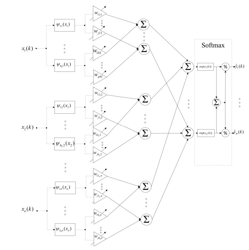
In the paper, we propose the modified generalized neo-fuzzy system. It is designed to solve the pattern-image recognition task by working with data that are fed to the system in the image form. The neo-fuzzy system can work with small training datasets, where classes can overlap in a features space. The core of the system under consideration is a modification of multidimensional generalized neuro-fuzzy neuron with an additional softmax activation function in the output layer instead of the defuzzification layer and quartic-kernel functions as membership ones. The learning procedure of the system combined cross-entropy criterion optimization using a matrix version of the optimal by speed Kaczmarz-Widrow-Hoff algorithm with the additional filtering (smoothing) properties. In comparison to the well-known systems, the modified neo-fuzzy one provides both numerical and computational implementation simplicity. The computational experiments have proved the effectiveness of the modified generalized neo-fuzzy-neuron, including the situation with shot training datasets.
Citation: Yevgeniy Bodyanskiy, Olha Chala, Natalia Kasatkina, Iryna Pliss. Modified generalized neo-fuzzy system with combined online fast learning in medical diagnostic task for situations of information deficit[J]. Mathematical Biosciences and Engineering, 2022, 19(8): 8003-8018. doi: 10.3934/mbe.2022374
In the paper, we propose the modified generalized neo-fuzzy system. It is designed to solve the pattern-image recognition task by working with data that are fed to the system in the image form. The neo-fuzzy system can work with small training datasets, where classes can overlap in a features space. The core of the system under consideration is a modification of multidimensional generalized neuro-fuzzy neuron with an additional softmax activation function in the output layer instead of the defuzzification layer and quartic-kernel functions as membership ones. The learning procedure of the system combined cross-entropy criterion optimization using a matrix version of the optimal by speed Kaczmarz-Widrow-Hoff algorithm with the additional filtering (smoothing) properties. In comparison to the well-known systems, the modified neo-fuzzy one provides both numerical and computational implementation simplicity. The computational experiments have proved the effectiveness of the modified generalized neo-fuzzy-neuron, including the situation with shot training datasets.

| [1] | C. L. Mumford, L. C. Jain, Computational Intelligence, Springer, Berlin Heidelberg, 2009. |
| [2] | R. Kruse, C. Borgelt, C. Braune, S. Mostaghim, M. Steinbrecher, Computational Intelligence, A Methodological Introduction, Springer-Verlag, Berlin, 2016. |
| [3] | J. Kacprzyk, W. Pedrycz, Springer Handbook of Computational Intelligence, Springer Verlag, Berlin Heidelberg, 2015. |
| [4] | P. Berka, J. Rauch, D. A. Zighed, Data Mining and Medical Knowledge Management: Cases and Applications, IGI Global, 2009. |
| [5] | R. Kountchev, B. Iantovics, Advances in Intelligent Analysis of Medical Data and Decision Support Systems, Springer International Publishing, Heidelberg, 2013. |
| [6] | Y. Bodyanskiy, I. Perova, O. Vynokurova, I. Izonin, Adaptive wavelet diagnostic neuro-fuzzy network for biomedical tasks, 14th International Conference on Advanced Trends in Radioelecrtronics, Telecommunications and Computer Engineering (TCSET), (2018), 711-715. https://doi.org/10.1109/TCSET.2018.8336299 |
| [7] | Y. Syerov, N. Shakhovska, S. Fedushko, Method of the data adequacy determination of personal medical profiles, in (Eds.), Advances in Artificial Systems for Medicine and Education Ⅱ (eds. Z. Hu, S. V. Petoukhov, M. He), Springer International Publishing, Cham, (2018), 333-343. |
| [8] | K. L. Du, M. N. S. Swamy, Neural Networks and Statistical Learning, Springer, London, 2013. |
| [9] |
J. Schmidhuber, Deep learning in neural networks: An overview, Neural Networks, 61 (2015), 85-117. https://doi.org/10.1016/j.neunet.2014.09.003 doi: 10.1016/j.neunet.2014.09.003

|
| [10] | I. Goodfellow, Y. Bengio, A. Courville, Deep Learning, MIT Press, United States, 2016. |
| [11] | P. V. C. Souza, Fuzzy neural networks and neuro-fuzzy networks: A review the main techniques and applications used in the literature, Appl. Soft Comput., 92 (2020), 106275. |
| [12] | D. Graupe, Deep Learning Neural Networks: Design and Case Studies, World Scientific, New Jersey, 2016. |
| [13] | R. Tkachenko, I. Izonin, P. Tkachenko, Neuro-Fuzzy Diagnostics Systems Based on SGTM Neural-Like Structure and T-Controller, in Lecture Notes in Computational Intelligence and Decision Making (eds. S. Babichev, V. Lytvynenko), Springer International Publishing, Cham, (2021), 685-695. https://doi.org/10.1007/978-3-030-82014-5_47 |
| [14] |
D. F. Specht, Probabilistic neural networks, Neural Network, 3 (1990), 109-118. https://doi.org/10.1016/0893-6080(90)90049-Q doi: 10.1016/0893-6080(90)90049-Q
|
| [15] |
D. F. Specht, Probabilistic neural networks and polynomial ADALINE as complementary techniques to classification, IEEE Trans. Neural Networks, 1 (1990), 111-121. https://doi.org/10.1109/72.80210 doi: 10.1109/72.80210
|
| [16] | O. Nelles, Nonlinear Systems Identification, Springer, Berlin, 2002. |
| [17] | D. R. Zahirniak, R. Chapman, S. K. Rogers, B. W. Suter, Pattern recognition using radial basis function network, Aerospace Appl. Artif. Intell., 1990 (1990), 249-260. |
| [18] | T. Yamakawa, A neo-fuzzy neuron and its application to system identification and prediction of the system behavior, in Proceedings of the 2nd International Conference on Fuzzy Logic and Neural Networks, (1992), 477-483. |
| [19] | E. Uchino, T. Yamakawa, Neo-fuzzy-neuron based new approach to system modeling, with application to actual system, in Proceedings Sixth International Conference on Tools with Artificial Intelligence, (1994), 564-570. https://doi.org/10.1109/TAI.1994.346442 |
| [20] | T. Miki, T. Yamakawa, Analog implementation of neo-fuzzy neuron and its on-board learning, Comput. Intell. Appl., 1999 (1999), 144-149. |
| [21] |
D. Zurita, M. Delgado, J. A. Carino, J. A. Ortega, G. Clerc, Industrial time series modelling by means of the neo-fuzzy neuron, IEEE Access, 4 (2016), 6151-6160. https://doi.org/10.1109/ACCESS.2016.2611649 doi: 10.1109/ACCESS.2016.2611649
|
| [22] | Y. Bodyanskiy, I. Kokshenev, V. Kolodyazhniy, An adaptive learning algorithm for a neo-fuzzy neuron, in Proceedings of the 3rd Conference of the European Society for Fuzzy Logic and Technology, (2003), 375-379. |
| [23] |
Y. Bodyanskiy, N. Kulishova, O. Chala, The extended multidimensional neo-fuzzy system and its fast learning in pattern recognition tasks, Data, 3 (2018), 63. https://doi.org/10.3390/data3040063 doi: 10.3390/data3040063
|
| [24] | R. P. Landim, B. Rodrigues, S. R. Silva, W. M. Caminhas, A neo-fuzzy-neuron with real time training applied to flux observer for an induction motor, in Proceedings 5th Brazilian Symposium on Neural Networks (Cat. No.98EX209), (1998), 67-72. https://doi.org/10.1109/SBRN.1998.730996 |
| [25] | E. Parzen, On estimation of a probability density function and mode, Ann. Math. Statist., 33 (1962), 1065-1076. |
| [26] |
S. Kaczmarz, Approximate solution of systems of linear equations, Int. J. Control, 57 (1993), 1269-1271. https://doi.org/10.1080/00207179308934446 doi: 10.1080/00207179308934446
|
| [27] | B. Widrow, M. E. Hoff, Adaptive switching circuits, Stanford University, Stanford Electronics Labs, California, 1960. |
| [28] | Y. Bodyanskiy, V. Kolodyazhniy, A. Stephan, An adaptive learning algorithm for a neuro-fuzzy network, in Computational Intelligence Theory and Applications Fuzzy Days, (2001), 68-75. https://doi.org/10.1007/3-540-45493-4_11 |
| [29] |
G. C. Goodwin, P. J. Ramadge, P. E. Caines, Discrete time stochastic adaptive control, SIAM J. Control Optim., 19 (1981), 829-853. https://doi.org/10.1137/0319052 doi: 10.1137/0319052
|
| [30] |
R. A. Adegbola, Childhood pneumonia as a global health priority and the strategic interest of the bill and melinda gates foundation, Clin. Infect. Dis., 54 (2012), S89-S92. https://doi.org/10.1093/cid/cir1051 doi: 10.1093/cid/cir1051
|
| [31] | D. Kermany, K. Zhang, M. Goldbaum, Labeled optical coherence tomography (OCT) and chest X-ray images for classification, Mendeley Data, 2 (2018). |
| [32] | Z. Camlica, H. R. Tizhoosh, F. Khalvati, Medical image classification via SVM using LBP features from saliency-based folded data, in 2015 IEEE 14th International Conference on Machine Learning and Applications (ICMLA), (2015), 128-132. |
| [33] | M. A. Khan, N. A. Syed, Image processing techniques for automatic detection of tumor in human brain using SVM, Int. J. Adv. Res. Comput. Commun. Eng., 4 (2015), 541-544. |
| [34] |
I. Izonin, A. Trostianchyn, Z. Duriagina, R. Tkachenko, T. Tepla, N. Lotoshynska, The combined use of the wiener polynomial and SVM for material classification task in medical implants production, Int. J. Intell. Syst. Appl., 10 (2018), 40-47. http://doi.org/10.5815/ijisa.2018.09.05 doi: 10.5815/ijisa.2018.09.05
|
| [35] | Q. Li, W. Cai, X. Wang, Y. Zhou, D. Feng, M. Chen, Medical image classification with convolutional neural network, in 2014 13th International Conference on Control Automation Robotics and Vision (ICARCV), (2014), 844-848. |
| [36] | X. Wang, Y. Peng, L. Lu, Z. Lu, M. Bagheri, R. M. Summers, ChestX-Ray8: Hospital-scale chest X-Ray database and benchmarks on weakly-supervised classification and localization of common thorax diseases, in 2017 IEEE Conference on Computer Vision and Pattern Recognition (CVPR), (2017), 2097-2106. https://doi.org/10.1109/CVPR.2017.369 |
| [37] |
O. Russakovsky, J. Deng, H. Su, J. Krause, S. Satheesh, S. Ma, et al., ImageNet large scale visual recognition challenge, Int. J. Comput. Vis., 115 (2015), 211-252. https://doi.org/10.1007/s11263-015-0816-y doi: 10.1007/s11263-015-0816-y
|
| [38] | T. Iesmantas, R. Alzbutas, Convolutional capsule network for classification of breast cancer histology images, in Image Analysis and Recognition, (2018), 853-860. https://doi.org/10.1007/978-3-319-93000-8_97 |
| [39] | P. Afshar, A. Mohammadi, K. N. Plataniotis, Brain tumor type classification via capsule networks, in 2018 25th IEEE International Conference on Image Processing (ICIP), (2018), 3129-3133. https://doi.org/10.1109/ICIP.2018.8451379 |
| [40] | A. Jiménez-Sánchez, S. Albarqouni, D. Mateus, Capsule networks against medical imaging data challenges, in Intravascular Imaging and Computer Assisted Stenting and Large-Scale Annotation of Biomedical Data and Expert Label Synthesis, (2018), 150-160. https://doi.org/10.1007/978-3-030-01364-6_17 |
| [41] | E. Xi, S. Bing, Y. Jin, Capsule network performance on complex data, preprint, arXiv: 171203480. |
| [42] |
M. Mahesh, The essential physics of medical imaging, Med. Phys., 40 (2013), 077301. https://doi.org/10.1118/1.4811156 doi: 10.1118/1.4811156
|
| [43] |
H. D. Tagare, C. C. Jaffe, J. Duncan, Medical image databases: A content-based retrieval approach, J. Am. Med. Inf. Assoc., 4 (1997), 184-198. https://doi.org/10.1136/jamia.1997.0040184 doi: 10.1136/jamia.1997.0040184
|
| [44] | S. J. Fong, G. Li, N. Dey, R. G. Crespo, E. Herrera-Viedma, Finding an accurate early forecasting model from small dataset: A case of 2019-nCoV Novel Coronavirus outbreak, preprint, arXiv: 2003.10776. |
Figures(5) / Tables(3)

Yevgeniy Bodyanskiy, Olha Chala, Natalia Kasatkina, Iryna Pliss. Modified generalized neo-fuzzy system with combined online fast learning in medical diagnostic task for situations of information deficit[J]. Mathematical Biosciences and Engineering, 2022, 19(8): 8003-8018. doi: 10.3934/mbe.2022374


 DownLoad: