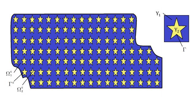
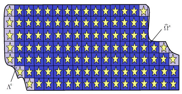
The first aim of this paper is to study, by means of the periodic unfolding method, the homogenization of elliptic problems with source terms converging in a space of functions less regular than the usual $ L^2 $, in an $ \varepsilon $-periodic two component composite with an imperfect transmission condition on the interface. Then we exploit this result to describe the asymptotic behaviour of the exact controls and the corresponding states of hyperbolic problems set in composites with the same structure and presenting the same condition on the interface. The exact controllability is developed by applying the Hilbert Uniqueness Method, introduced by J. -L. Lions, which leads us to the construction of the exact controls as solutions of suitable transposed problem.
Citation: Sara Monsurrò, Carmen Perugia. Homogenization and exact controllability for problems with imperfect interface[J]. Networks and Heterogeneous Media, 2019, 14(2): 411-444. doi: 10.3934/nhm.2019017
The first aim of this paper is to study, by means of the periodic unfolding method, the homogenization of elliptic problems with source terms converging in a space of functions less regular than the usual $ L^2 $, in an $ \varepsilon $-periodic two component composite with an imperfect transmission condition on the interface. Then we exploit this result to describe the asymptotic behaviour of the exact controls and the corresponding states of hyperbolic problems set in composites with the same structure and presenting the same condition on the interface. The exact controllability is developed by applying the Hilbert Uniqueness Method, introduced by J. -L. Lions, which leads us to the construction of the exact controls as solutions of suitable transposed problem.

| [1] |
Macroscopic modelling of heat transfer in composites with interfacial thermal barrier. Internat. J. Heat Mass Transfer (1994) 37: 2885-2892. 
|
| [2] | A. Bensoussan, J. L. Lions and G. Papanicolaou, Asymptotic Analysis for Periodic Structures, North-Holland, Amsterdam, 1978. |
| [3] | Homogenization of diffusion in composite media with interfacial barrier. Rev. Roumaine Math. Pures Appl. (1999) 44: 23-36. |
| [4] | Estimates in homogenization of degenerate elliptic equations by spectral method. Asymptot. Anal. (2013) 81: 189-209. |
| [5] | (1947) Conduction of Heat in Solids. Oxford: At the Clarendon Press. |
| [6] |
D. Cioranescu, A. Damlamian and G. Griso, The periodic unfolding method in homogenization, SIAM J. Math. Anal., 40 (2008), 1585–1620. doi: 10.1137/080713148
|
| [7] |
The periodic unfolding method in domains with holes. SIAM J. Math. Anal. (2012) 44: 718-760.
|
| [8] | Exact internal controllability in perforated domains. J. Math. Pures. Appl (1989) 68: 185-213. |
| [9] | (1999) An Introduction to Homogenization. New York: Oxford Lecture Ser. Math., Appl. 17, Oxford University Press. |
| [10] | The periodic unfolding method in perforated domains. Portugaliae Mathematica (2006) 63: 467-496. |
| [11] | Exact boundary controllability for the wave equation in domains with small holes. J. Math. Pures. Appl. (1992) 71: 343-377. |
| [12] |
Homogenization in open sets with holes. J. Math. Anal. Appl. (1979) 71: 590-607.
|
| [13] |
Asymptotic behaviour and correctors for linear Dirichlet problems with simultaneously varying operators and domains. Ann. I. H. Poincaré (2004) 21: 445-486.
|
| [14] |
Optimal control for a parabolic problem in a domain with higly oscillating boundary. Appl. Anal. (2004) 83: 1245-1264.
|
| [15] |
Optimal control problem for an anisotropic parabolic problem in a domain with very rough boundary. Ric. Mat. (2014) 63: 307-328.
|
| [16] |
Optimal control for a second-order linear evolution problem in a domain with oscillating boundary. Complex Var. Elliptic Equ. (2015) 6: 1392-1410.
|
| [17] | Exact internal controllability for a hyperbolic problem in a domain with highly oscillating boundary. Asymptot. Anal. (2013) 83: 189-206. |
| [18] |
Exact internal controllability for the wave equation in a domain with oscillating boundary with Neumann boundary condition. Evol. Equ. Control Theory (2015) 4: 325-346.
|
| [19] | Some corrector results for composites with imperfect interface. Rend. Mat. Ser. Ⅶ (2006) 26: 189-209. |
| [20] |
P. Donato, Homogenization of a class of imperfect transmission problems, in Multiscale Problems: Theory, Numerical Approximation and Applications doi: 10.1142/9789814366892_0001
|
| [21] |
Homogenization of the wave equation in composites with imperfect interface: A memory effect. J. Math. Pures Appl. (2007) 87: 119-143.
|
| [22] |
Correctors for the homogenization of a class of hyperbolic equations with imperfect interfaces. SIAM J. Math. Anal. (2009) 40: 1952-1978.
|
| [23] |
Corrector results for a parabolic problem with a memory effect. ESAIM: Math. Model. Numer. Anal. (2010) 44: 421-454.
|
| [24] |
Asymptotic behavior of the approximate controls for parabolic equations with interfacial contact resistance. ESAIM Control Optim. Calc. Var. (2015) 21: 138-164.
|
| [25] | Approximate controllability of a parabolic system with imperfect interfaces. Philipp. J. Sci. (2015) 144: 187-196. |
| [26] |
The periodic unfolding method for a class of imperfect trasmission problems. J. Math. Sci. (2011) 176: 891-927.
|
| [27] |
Homogenization of diffusion problems with a nonlinear interfacial resistance. Nonlinear Differ. Equ. Appl. (2015) 22: 1345-1380.
|
| [28] |
Homogenization of two heat conductors with interfacial contact resistance. Anal. Appl. (2004) 2: 247-273.
|
| [29] |
Homogenization of a class of singular elliptic problems in perforated domains. Nonlinear Anal. (2018) 173: 180-208.
|
| [30] |
Approximate controllability of linear parabolic equations in perforated domains. ESAIM Control Optim. Calc. Var. (2001) 6: 21-38.
|
| [31] |
Homogenization and behaviour of optimal controls for the wave equation in domains with oscillating boudary. Nonlinear Differ. Equ. Appl. (2007) 14: 455-489.
|
| [32] |
Asymptotic analysis of an optimal control problem involving a thick two-level junction with alternate type of controls. J. Optim. Th. and Appl. (2010) 144: 205-225.
|
| [33] |
Homogenization of quasilinear optimal control problems involving a thick multilevel junction of type 3:2:1. ESAIM Control Optim. Calc. Var. (2012) 18: 583-610.
|
| [34] |
L. Faella and S. Monsurrò, Memory effects arising in the homogenization of composites with inclusions, in Topics on Mathematics for Smart System doi: 10.1142/9789812706874_0008
|
| [35] | Homogenization of imperfect transmission problems: The case of weakly converging data. Differential Integral Equations (2018) 31: 595-620. |
| [36] |
Exact controllability for an imperfect transmission problem. J. Math. Pures Appl. (2019) 122: 235-271.
|
| [37] |
L. Faella and C. Perugia, Homogenization of a Ginzburg-Landau problem in a perforated domain with mixed boundary conditions, Bound. Value Probl., 2014 (2014), 28pp. doi: 10.1186/s13661-014-0223-2
|
| [38] |
L. Faella and C. Perugia, Optimal control for evolutionary imperfect transmission problems, Bound. Value Probl., 2015 (2015), 16pp. doi: 10.1186/s13661-015-0310-z
|
| [39] |
Optimal control for a hyperbolic problem in composites with imperfect interface: A memory effect. Evol. Equ. Control Theory (2017) 6: 187-217.
|
| [40] |
Null controllability of the semilinear heat equation. ESAIM Control Optim. Calc. Var. (1997) 2: 87-103.
|
| [41] |
Homogenization for heat transfer in polycristals with interfacial resistances. Appl. Anal. (2000) 75: 403-424.
|
| [42] |
A. M. Khludnev, L. Faella and C. Perugia, Optimal control of rigidity parameters of thin inclusions in composite materials, Z. Angew. Math. Phys., 68 (2017), Art. 47, 12 pp. doi: 10.1007/s00033-017-0792-x
|
| [43] |
Exact controllability for semilinear wave equations. J. Math. Anal. Appl. (2000) 250: 589-597.
|
| [44] | Contrôlabilité Exacte et Homogénéisation, I. Asymptotic Anal. (1988) 1: 3-11. |
| [45] | J. L. Lions, Contrôlabilité Exacte, Stabilization at Perturbations De Systéms Distributé, Tomes 1, 2, Massonn, RMA, 829, 1988. |
| [46] | J. L. Lions and E. Magenes, Non-homogeneous Boundary Value Problems and Applications, Vol I, Springer-Verlag Berlin Heidelberg, New York, 1972. |
| [47] |
Heat conduction in fine scale mixtures with interfacial contact resistance. SIAM J. Appl. Math. (1998) 58: 55-72.
|
| [48] |
Composite with imperfect interface. Proc. R. Soc. Lond. Ser. A (1996) 452: 329-358.
|
| [49] | Homogenization of a two-component composite with interfacial thermal barrier. Adv. Math. Sci. Appl. (2003) 13: 43-63. |
| [50] | Erratum for the paper "Homogenization of a two-component composite with interfacial thermal barrier". Adv. Math. Sci. Appl. (2004) 14: 375-377. |
| [51] | S. Monsurrò, Homogenization of a composite with very small inclusions and imperfect interface, in Multiscale problems and asymptotic analysis, GAKUTO Internat. Ser. Math. Sci. Appl., 24, Gakkotosho, Tokyo, (2006), 217–232. |
| [52] |
Homogenization of low-cost control problems on perforated domains. J. Math. Anal. Appl. (2009) 351: 29-42.
|
| [53] |
Asymptotic analysis of Neumann periodic optimal boundary control problem. Math. Methods Appl. Sci. (2016) 39: 4354-4374.
|
| [54] |
Homogenization and correctors for the hyperbolic problems with imperfect interfaces via the periodic unfolding method. Commun. Pure Appl. Anal. (2014) 13: 249-272.
|
| [55] |
The periodic unfolding method for a class of parabolic problems with imperfect interfaces. ESAIM Math. Model. Numer. Anal. (2014) 48: 1279-1302.
|
| [56] | E. Zuazua, Exact boundary controllability for the semilinear wave equation, in Nonlinear Partial Differential Equations and Their Applications, Collège de France Seminar, Vol. X (Paris, 1987–1988), Pitman Res. Notes Math. Ser., 220, Longman Sci. Tech., Harlow, 1991, 357–391. |
| [57] | Approximate controllability for linear parabolic equations with rapidly oscillating coefficients. Control Cybernet. (1994) 23: 793-801. |
| [58] |
Controllability of partial differential equations and its semi-discrete approximations. Discrete Contin. Dyn. Syst. (2002) 8: 469-513.
|
Figures(2)
Sara Monsurrò, Carmen Perugia. Homogenization and exact controllability for problems with imperfect interface[J]. Networks and Heterogeneous Media, 2019, 14(2): 411-444. doi: 10.3934/nhm.2019017


 DownLoad: