Crystalline evolutions in chessboard-like microstructures

Annalisa Malusa; Matteo Novaga; Annalisa Malusa; Matteo Novaga

doi:10.3934/nhm.2018022

Networks and Heterogeneous Media

2018, Volume 13, Issue 3: 493-513. doi: 10.3934/nhm.2018022

Previous Article Next Article

Crystalline evolutions in chessboard-like microstructures

Annalisa Malusa ^{1
,},
Matteo Novaga ^{2
,}

1.
Dipartimento di Matematica, Sapienza Università di Roma, Piazzale Aldo Moro 2, 00185 Roma, Italy
2.
Dipartimento di Matematica, Università di Pisa, Largo B. Pontecorvo 5, 56217 Pisa, Italy

Received: 01 November 2017 Revised: 01 March 2018
Primary: 53C44; Secondary: 35B27

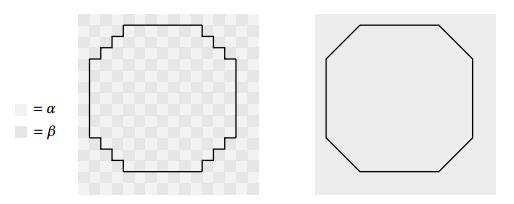
We describe the macroscopic behavior of evolutions by crystalline curvature of planar sets in a chessboard-like medium, modeled by a periodic forcing term. We show that the underlying microstructure may produce both pinning and confinement effects on the geometric motion.
- Geometric evolutions,
- crystalline flows,
- homogenization,
- facet–breaking,
- pinning
Citation: Annalisa Malusa, Matteo Novaga. Crystalline evolutions in chessboard-like microstructures[J]. Networks and Heterogeneous Media, 2018, 13(3): 493-513. doi: 10.3934/nhm.2018022

Related Papers:

Abstract

We describe the macroscopic behavior of evolutions by crystalline curvature of planar sets in a chessboard-like medium, modeled by a periodic forcing term. We show that the underlying microstructure may produce both pinning and confinement effects on the geometric motion.

References

[1]	Flat flow is motion by crystalline curvature for curves with crystalline energies. J. Differential Geometry (1995) 42: 1-22.
[2]	Homogenization of fronts in highly heterogeneous media. SIAM J. Math. Anal. (2011) 43: 212-227.
[3]	Approximation to driven motion by crystalline curvature in two dimensions. Adv. Math. Sci. and Appl. (2000) 10: 467-493.
[4]	Characterization of facet breaking for nonsmooth mean curvature flow in the convex case. Interfaces Free Bound. (2001) 3: 415-446.
[5]	On a crystalline variational problem, part Ⅰ: First variation and global $L^∞$ regularity. Arch. Rational Mech. Anal (2001) 57: 165-191.
[6]	On a crystalline variational problem, part Ⅱ: $BV$ regularity and structure of minimizers on facets. Arch. Rational Mech. Anal. (2001) 157: 193-217.
[7]	A. Braides, $Γ$-convergence for Beginners, Oxford University Press, 2002. doi: 10.1093/acprof:oso/9780198507840.001.0001
[8]	A. Braides, Local Minimization, Variational Evolution and Γ–convergence, Lecture Notes in Mathematics, Springer, Berlin, 2014. doi: 10.1007/978-3-319-01982-6
[9]	Crystalline Motion of Interfaces Between Patterns. J. Stat. Phys. (2016) 165: 274-319.
[10]	Motion and pinning of discrete interfaces. Arch. Ration. Mech. Anal. (2010) 195: 469-498.
[11]	A. Braides, A. Malusa and M. Novaga, Crystalline evolutions with rapidly oscillating forcing terms, to appear on Ann. Scuola Norm. Sci. doi: 10.2422/2036-2145.201707_011
[12]	Motion of discrete interfaces in periodic media. Interfaces Free Bound. (2013) 15: 451-476.
[13]	Motion of discrete interfaces through mushy layers. J. Nonlinear Sci. (2016) 26: 1031-1053.
[14]	Homogenization of a semilinear heat equation. J. Éc. polytech. Math. (2017) 4: 633-660.
[15]	Curve shortening flow in heterogeneous media. Interfaces and Free Bound. (2011) 13: 485-505.
[16]	Existence and uniqueness for a crystalline mean curvature flow. Comm. Pure Appl. Math. (2017) 70: 1084-1114.
[17]	A. Chambolle, M. Morini, M. Novaga and M. Ponsiglione, Existence and uniqueness for anisotropic and crystalline mean curvature flows, preprint, arXiv: 1702.03094.
[18]	Approximation of the anisotropic mean curvature flow. Math. Models Methods Appl. Sci. (2007) 17: 833-844.
[19]	Discontinuous Dynamical Systems: A tutorial on solutions, nonsmooth analysis, and stability. IEEE Control Systems Magazine (2008) 28: 36-73.
[20]	A. F. Filippov, Differential Equations with Discontinuous Righthand Sides, vol. 18 of Mathematics and Its Applications. Dordrecht, The Netherlands, Kluwer Academic Publishers, 1988. doi: 10.1007/978-94-015-7793-9
[21]	Y. Giga, Surface Evolution Equations. A Level Set Approach, vol. 99 of Monographs in Mathematics. Birkhäuser Verlag, Basel, 2006.
[22]	A comparison theorem for crystalline evolution in the plane. Quarterly of Applied Mathematics (1996) 54: 727-737.
[23]	Facet bending in the driven crystalline curvature flow in the plane. J. Geom. Anal. (2008) 18: 109-147.
[24]	Facet bending driven by the planar crystalline curvature with a generic nonuniform forcing term. J. Differential Equations (2009) 246: 2264-2303.
[25]	M. E. Gurtin, Thermomechanics of Evolving Phase Boundaries in the Plane, Oxford Mathematical Monographs. The Clarendon Press, Oxford University Press, New York, 1993.
[26]	Closed curves of prescribed curvature and a pinning effect. Netw. Heterog. Media (2011) 6: 77-88.
[27]	Crystalline variational problems. Bull. Amer. Math. Soc. (1978) 84: 568-588.
[28]	Geometric Models of Crystal Growth. Acta Metall. Mater. (1992) 40: 1443-1474.

Reader Comments

Your name:*

Email:*
© 2018 the Author(s), licensee AIMS Press. This is an open access article distributed under the terms of the Creative Commons Attribution License (http://creativecommons.org/licenses/by/4.0)