A contiunous-time $ SIS $ criss-cross model of co-infection in a heterogeneous population

Marcin Choiński; Marcin Choiński

doi:10.3934/mbe.2025038

Mathematical Biosciences and Engineering

2025, Volume 22, Issue 5: 1055-1080. doi: 10.3934/mbe.2025038

Previous Article Next Article

Research article Special Issues

A contiunous-time $ SIS $ criss-cross model of co-infection in a heterogeneous population

Marcin Choiński ^,

Institute of of Information Technology, Warsaw University of Life Sciences – SGGW, Nowoursynowska 159 Street, building 34, 02-776 Warsaw, Poland

Academic Editor: Glenn Ledder

Received: 03 January 2025 Revised: 11 March 2025 Accepted: 17 March 2025 Published: 21 March 2025

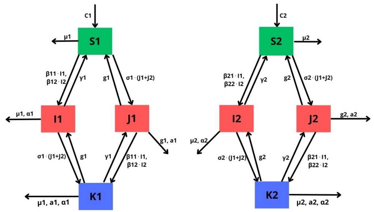
In this paper, we introduce and analyze a contiunous-time model of co-infection dynamics in a heterogeneous population consisting of two subpopulations that differ in the risk of getting infected by individuals with two diseases. We assume that each parameter reflecting a given process for each subpopulation has different values, which makes the population completely heterogeneous. Such complexity and the population heterogeneity make our paper unique, reflecting co-infection dynamics. Moreover, we establish an epidemic spread for each disease not only in a sole subpopulation but also with criss-cross transmission, meaning between different subpopulations. The proposed system has a disease-free stationary state and two states reflecting the presence of one disease. We indicate conditions for their existence and local stability. The conditions for the local stability for states reflecting one disease have a complicated form, so we strengthened them so that they are more transparent. Investigation on the existence of a postulated endemic state corresponding to both disease's presence leads to a complex analysis, which is why we only provide an insight on this issue. Here, we also provide the basic reproduction number of our model and investigate properties of this number. The system has a universal structure; as such, it can be applied to investigate co-infection of different infectious diseases.
- co-infection,
- $ SIS $ model,
- local stability,
- population heterogeneity,
- dynamical systems
Citation: Marcin Choiński. A contiunous-time $ SIS $ criss-cross model of co-infection in a heterogeneous population[J]. Mathematical Biosciences and Engineering, 2025, 22(5): 1055-1080. doi: 10.3934/mbe.2025038

Related Papers:

Abstract

In this paper, we introduce and analyze a contiunous-time model of co-infection dynamics in a heterogeneous population consisting of two subpopulations that differ in the risk of getting infected by individuals with two diseases. We assume that each parameter reflecting a given process for each subpopulation has different values, which makes the population completely heterogeneous. Such complexity and the population heterogeneity make our paper unique, reflecting co-infection dynamics. Moreover, we establish an epidemic spread for each disease not only in a sole subpopulation but also with criss-cross transmission, meaning between different subpopulations. The proposed system has a disease-free stationary state and two states reflecting the presence of one disease. We indicate conditions for their existence and local stability. The conditions for the local stability for states reflecting one disease have a complicated form, so we strengthened them so that they are more transparent. Investigation on the existence of a postulated endemic state corresponding to both disease's presence leads to a complex analysis, which is why we only provide an insight on this issue. Here, we also provide the basic reproduction number of our model and investigate properties of this number. The system has a universal structure; as such, it can be applied to investigate co-infection of different infectious diseases.

References

[1]	L. Almeida, P. A. Bliman, G. Nadin, B. Perthame, N. Vauchelet, Final size and convergence rate for an epidemic in heterogeneous population, Math. Models Methods Appl. Sci., 31 (2021), 1021–1051. https://doi.org/10.1142/S0218202521500251 doi: 10.1142/S0218202521500251
[2]	G. Ellison, Implications of heterogeneous SIR models for analyses of COVID-19, Rev. Econ. Design, 28 (2024), 651–687. https://doi.org/10.1007/s10058-024-00355-z doi: 10.1007/s10058-024-00355-z
[3]	X. Yan, K. Li, Z. Lei, J. Luo, Q. Wang, S. Wei, Prevalence and associated outcomes of coinfection between SARS-CoV-2 and influenza: a systematic review and meta-analysis, Int. J. Infect. Dis., 136 (2023), 29–36. https://doi.org/10.1016/j.ijid.2023.08.021 doi: 10.1016/j.ijid.2023.08.021
[4]	J. Sandlund, P. Naucler, S. Dashti, A. Shokri, S. Eriksson, M. Hjertqvist, et al., Bacterial coinfections in travelers with malaria: rationale for antibiotic therapy, J. Clin. Microbiol., 51 (2013), 15–21. https://doi.org/10.1128/JCM.02149-12 doi: 10.1128/JCM.02149-12
[5]	R. B. Birger, R. D. Kouyos, T. Cohen, E. C. Griffiths, S. Huijben, M. J. Mina, et al., The potential impact of coinfection on antimicrobial chemotherapy and drug resistance, Trends Microbiol., 23 (2015), 537–544. https://doi.org/10.1016/j.tim.2015.05.002 doi: 10.1016/j.tim.2015.05.002
[6]	J. Marcinkiewicz, Increase in the incidence of invasive bacterial infections following the COVID-19 pandemic: potential links with decreased herd trained immunity – a novel concept in medicine, Pol. Arch. Intern. Med., 134 (2024), 16794. https://doi.org/10.20452/pamw.16794 doi: 10.20452/pamw.16794
[7]	A. Sophonsri, C. Kelsom, M. Lou, P. Nieberg, A. Wong-Beringer, Risk factors and outcome associated with coinfection with carbapenem–resistant Klebsiella pneumoniae and carbapenem–resistant Pseudomonas aeruginosa or Acinetobacter baumanii: a descriptive analysis, Front. Cell. Infect. Microbiol., 13 (2023), 1231740. https://doi.org/10.3389/fcimb.2023.1231740 doi: 10.3389/fcimb.2023.1231740
[8]	L. R. Idrus, N. Fitria, F. D. Purba, J. W. C. Alffenaar, M. J. Postma, Analysis of health-related quality of life and incurred costs among human immunodeficiency virus, tuberculosis, and tuberculosis/HIV coinfected outpatients in Indonesia, Value Health Reg. Issues, 41 (2024), 32–40. https://doi.org/10.1016/j.vhri.2023.10.010. doi: 10.1016/j.vhri.2023.10.010
[9]	D. L. Silva, C. M. Lima, V. C. R. Magalhaes, L. M. Baltazar, N. T. A. Peres, R. B. Caligiorne, et al., Fungal and bacterial coinfections increase mortality of severely ill COVID-19 patients, J. Hosp. Infect., 113 (2021), 145–154. https://doi.org/10.1016/j.jhin.2021.04.001 doi: 10.1016/j.jhin.2021.04.001
[10]	F. Inayaturohmat, N. Anggriani, A. K. Supriatna, M. H. A. Biswas, A systematic literature review of mathematical models for coinfections: tuberculosis, malaria, and HIV/AIDS, J. Multidiscip. Healthcare, 2024 (2024), 1091–1109. https://doi.org/10.2147/JMDH.S446508 doi: 10.2147/JMDH.S446508
[11]	J. Li, L. Wang, H. Zhao, Z. Ma, Dynamical behavior of an epidemic model with coinfection of two diseases, Rocky Mt. J. Math., 38 (2008), 1457–1479. https://doi.org/10.1216/RMJ-2008-38-5-1457 doi: 10.1216/RMJ-2008-38-5-1457
[12]	K. G. Mekonen, L. L. Obsu, Mathematical modeling and analysis for the co-infection of COVID–19 and tuberculosis, Heliyon, 8 (2022). https://doi.org/10.1016/j.heliyon.2022.e11195
[13]	F. Inayaturohmat, N. Anggriani, A. K. Supriatna, A mathematical model of tuberculosis and COVID-19 coinfection with the effect of isolation and treatment, Front. Appl. Math. Stat., 8 (2022), 958081. https://doi.org/10.3389/fams.2022.958081 doi: 10.3389/fams.2022.958081
[14]	A. Din, S. Amine, A. Allali, A stochastically perturbed co-infection epidemic model for COVID–19 and hepatitis B virus, Nonlinear Dyn., 111 (2023), 1921–1945. https://doi.org/10.1007/s11071-022-07899-1 doi: 10.1007/s11071-022-07899-1
[15]	A. M. Elaiw, A. S. Shflot, A. D. Hobiny, Stability analysis of SARS-CoV-2/HTLV-I coinfection dynamics model, Mathematics, 8 (2022), 6136–6166. https://doi.org/10.3934/math.2023310 doi: 10.3934/math.2023310
[16]	M. A. Hye, M. H. A. Biswas, M. F. Uddin, M. M. Rahman, A mathematical model for the transmission of co-infection with COVID-19 and kidney disease, Sci. Rep., 14 (2024), 5680. https://doi.org/10.1038/s41598-024-56399-2 doi: 10.1038/s41598-024-56399-2
[17]	E. F. Obiajulu, A. Omame, S. C. Inyama, U. H. Diala, S. A. AlQahtani, M. S. Al-Rakhami, et al., Analysis of a non-integer order mathematical model for double strains of dengue and COVID–19 co-circulation using an efficient finite-difference method, Sci. Rep., 13 (2023), 17787. https://doi.org/10.1038/s41598-023-44825-w doi: 10.1038/s41598-023-44825-w
[18]	J. Bruchfeld, M. Correia-Neves, G. Kaellenius, Tuberculosis and HIV coinfection, Cold Spring Harbor Perspect. Med., 4 (2015), a017871. https://doi.org/10.1101/cshperspect.a017871 doi: 10.1101/cshperspect.a017871
[19]	S. W. Teklu, Y. F. Abebaw, B. B. Terefe, D. K. Mamo, HIV/AIDS and TB co-infection deterministic model bifurcation and optimal control analysis, Inf. Med. Unlocked, 41 (2023), 101328. https://doi.org/10.1016/j.imu.2023.101328 doi: 10.1016/j.imu.2023.101328
[20]	T. K. Ayele, E. F. Doungmo Goufo, S. Mugisha, Co-infection mathematical model for HIV/AIDS and tuberculosis with optimal control in Ethiopia, PLoS One, 19 (2024), e0312539. https://doi.org/10.1371/journal.pone.0312539 doi: 10.1371/journal.pone.0312539
[21]	F. Dayan, N. Ahmed, A. Bariq, A. Akgül, M. Jawaz, M. Rafq, et al., Computational study of a co-infection model of HIV/AIDS and hepatitis C virus models, Sci. Rep., 13 (2023), 21938. https://doi.org/10.1038/s41598-023-48085-6 doi: 10.1038/s41598-023-48085-6
[22]	R. I. Gweryina, C. E. Madubueze, V. P. Bajiya, F. E. Esla, Modeling and analysis of tuberculosis and pneumonia co-infection dynamics with cost-effective strategies, Results Control Optim., 10 (2023), 100210. https://doi.org/10.1016/j.rico.2023.100210 doi: 10.1016/j.rico.2023.100210
[23]	M. Choiński, M. Bodzioch, U. Foryś, Simple criss-cross model of epidemic for heterogeneous populations, Commun. Nonlinear Sci. Numer. Simul., 79 (2019), 104920. https://doi.org/10.1016/j.cnsns.2019.104920 doi: 10.1016/j.cnsns.2019.104920
[24]	M. Bodzioch, M. Choiński, U. Foryś, $SIS$ criss-cross model of tuberculosis in heterogeneous population, Discrete Contin. Dyn. Syst. - Ser. B, 24 (2019), 2169–2188. https://doi.org/10.3934/dcdsb.2019089 doi: 10.3934/dcdsb.2019089
[25]	J. Romaszko, A. Siemaszko, M. Bodzioch, A. Buciński, A. Doboszyńska, Active case finding among homeless people as a means of reducing the incidence of pulmonary tuberculosis in general population, Adv. Exp. Med. Biol., 911 (2016), 67–76. https://doi.org/10.1007/5584_2016_225 doi: 10.1007/5584_2016_225
[26]	P. van den Driessche, J. Watmough, Reproduction numbers and sub-threshold endemic equilibria for compartmental models of disease transmission, Math. Biosci., 180 (2002), 29–48. https://doi.org/10.1016/S0025-5564(02)00108-6 doi: 10.1016/S0025-5564(02)00108-6
[27]	MathWorks, ode45, 2006. Available from: https://www.mathworks.com/help/matlab/ref/ode45.html. last access: 18th February, 2005.

Reader Comments

Your name:*

Email:*
© 2025 the Author(s), licensee AIMS Press. This is an open access article distributed under the terms of the Creative Commons Attribution License (http://creativecommons.org/licenses/by/4.0)