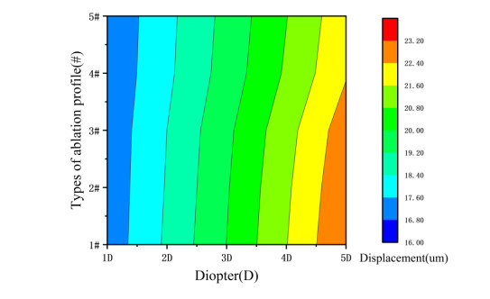
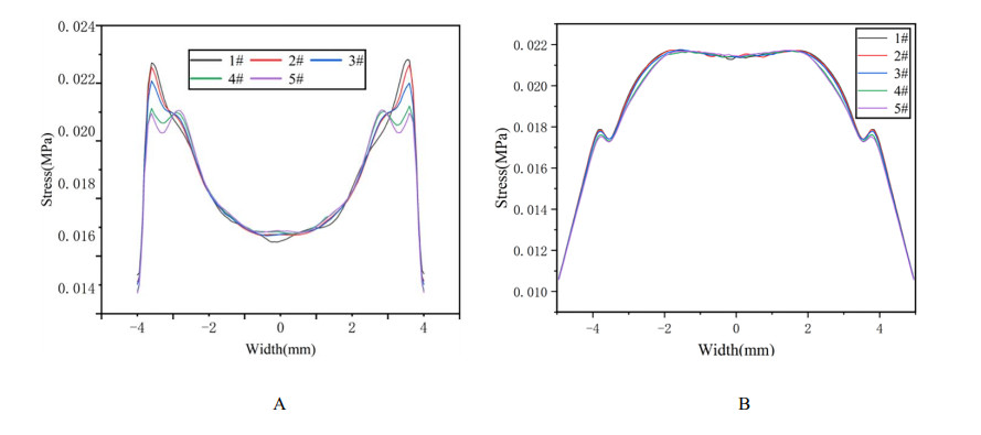
We studied the effects of the aspheric transition zone on the optical wavefront aberrations, corneal surface displacement, and stress induced by the biomechanical properties of the cornea after conventional laser in situ keratomileusis (LASIK) refractive surgery. The findings in this study can help improve visual quality after refractive surgery. Hyperopia correction in 1-5D was simulated using five types of aspheric transition zones with finite element modeling. The algorithm for the simulations was designed according to the optical path difference. Wavefront aberrations were calculated from the displacements on the anterior and posterior corneal surfaces. The vertex displacements and stress on the corneal surface were also evaluated. The results showed that the aspheric transition zone has an effect on the postoperative visual quality. The main wavefront aberrations on the anterior corneal surface are defocus, y-primary astigmatism, x-coma, and spherical aberrations. The wavefront aberrations on the corneal posterior surface were relatively small and vertex displacements on the posterior corneal surface were not significantly affected by the aspheric transition zone. Stress analysis revealed that the stress on the cutting edge of the anterior corneal surface decreased with the number of aspheric transition zone increased, and profile #1 resulted in the maximum stress. The stress on the posterior surface of the cornea was more concentrated in the central region and was less than that on the anterior corneal surface overall. The results showed that the aspheric transition zone has an effect on postoperative aberrations, but wavefront aberrations cannot be eliminated. In addition, the aspheric transition zone influences the postoperative biomechanical properties of the cornea, which significantly affect the postoperative visual quality.
Citation: Ruirui Du, Lihua Fang, Binhui Guo, Yinyu Song, Huirong Xiao, Xinliang Xu, Xingdao He. Simulated biomechanical effect of aspheric transition zone ablation profiles after conventional hyperopia refractive surgery[J]. Mathematical Biosciences and Engineering, 2021, 18(3): 2442-2454. doi: 10.3934/mbe.2021124
We studied the effects of the aspheric transition zone on the optical wavefront aberrations, corneal surface displacement, and stress induced by the biomechanical properties of the cornea after conventional laser in situ keratomileusis (LASIK) refractive surgery. The findings in this study can help improve visual quality after refractive surgery. Hyperopia correction in 1-5D was simulated using five types of aspheric transition zones with finite element modeling. The algorithm for the simulations was designed according to the optical path difference. Wavefront aberrations were calculated from the displacements on the anterior and posterior corneal surfaces. The vertex displacements and stress on the corneal surface were also evaluated. The results showed that the aspheric transition zone has an effect on the postoperative visual quality. The main wavefront aberrations on the anterior corneal surface are defocus, y-primary astigmatism, x-coma, and spherical aberrations. The wavefront aberrations on the corneal posterior surface were relatively small and vertex displacements on the posterior corneal surface were not significantly affected by the aspheric transition zone. Stress analysis revealed that the stress on the cutting edge of the anterior corneal surface decreased with the number of aspheric transition zone increased, and profile #1 resulted in the maximum stress. The stress on the posterior surface of the cornea was more concentrated in the central region and was less than that on the anterior corneal surface overall. The results showed that the aspheric transition zone has an effect on postoperative aberrations, but wavefront aberrations cannot be eliminated. In addition, the aspheric transition zone influences the postoperative biomechanical properties of the cornea, which significantly affect the postoperative visual quality.

| [1] | Z. W. Shen, H. Z. Zhou, H. Yin, J. T. Wu, L. Li, Fine adjusted-customized ablation LASIK treatment for myopia, Int. J. Ophthalmol., 5 (2005), 1194-1197. |
| [2] | Z. J. Fan, S. J. Xu, Z. H. Jia, B. C. Liu, Clinical significance of corneal Q value in myopic patients, Int. J. Ophthalmol., 6 (2006), 642-643. |
| [3] | X. U. Li, Q. Tao, L. Y. Zhuang, Visual outcome after optimized aspheric transitionzone laser keratomileusis compared toconventional LASIK, Int. Eye Sci., 7 (2007), 623-625. |
| [4] |
S. MacRae, Excimer ablation design and elliptical transition zones, J. Cataract Refractive Surg., 25 (1999), 1191-1197. doi: 10.1016/S0886-3350(99)00144-3

|
| [5] |
L. Fang, Y. Wang, X. He, Theoretical analysis of wavefront aberration caused by treatment decentration and transition zone after custom myopic laser refractive surgery, J. Cataract Refractive Surg., 39 (2013), 1336-1347. doi: 10.1016/j.jcrs.2013.03.020
|
| [6] |
G. M. Dai, Application of complementary error function to the transition zone of myopic ablation shapes in refractive surgery, J. Appl. Math. Phys., 5 (2017), 1521-1528. doi: 10.4236/jamp.2017.58125
|
| [7] | E. Gross, R. Hofer, J. Wong, Application of blend zones, depth reduction, and transition zones to ablation shapes, Patent No. 8216213, 2012. |
| [8] | J. Shen, Y. Zhang, W. Liao, Mathematical model based corneal toric surface for excimer laser refractive surgery, J. Southeast Univ., 36 (2006), 531-536. |
| [9] |
M. J. Endl, C. E. Martinez, S. D. Klyce, M. B. McDonald, S. J. Coorpender, R. A. Applegate, et al., Effect of larger ablation zone and transition zone on corneal optical aberrations after photorefractive keratectomy, Arch. Ophthalmol., 119 (2001), 1159-1164. doi: 10.1001/archopht.119.8.1159
|
| [10] | I. B. Damgaard, M. Ang, A. M. Mahmoud, M. Farook, C. J. Roberts, J. S. Mehta, Functional optical zone and centration following SMILE and LASIK: a prospective, randomized, contralateral eye study, J. Refractive Surg., 35 (2019), 230-237. |
| [11] | A. P. Nisarta, D. Desai, K. Solanki, Corneal higher order aberrations after aspheric LASIK treatment, Int. J. Health Sci. Res., 6 (2016), 107-113. |
| [12] | T. Gamaly, LASIK with the optimized aspheric transition zone and cross-cylinder technique for the treatment of astigmatism from 1.00 to 4.25 diopters, J. Refractive Surg., 25 (2009), S927-930. |
| [13] |
Y. H. Komai, I. Toda, N. A. Kato, M. Ito, T. Yamaoto, K. Tsubota, Comparison of LASIK using the NIDEK EC-5000 optimized aspheric transition zone (OATz) and conventional ablation profile, J. Refractive Surg., 22 (2006), 546-555. doi: 10.3928/1081-597X-20060601-06
|
| [14] | M. Hantera, Comparison of postoperative wavefront aberrations after NIDEK CXIII optimized aspheric transition zone treatment and OPD-guided custom aspheric treatment, J. Refractive Surg., 25 (2009), S922-926. |
| [15] | M. Balidis, Biomechanical profile of refractive surgery procedures, Acta Ophthalmol., 97 (2019). |
| [16] | G. V. Voronin, I. A. Bubnova, Changes in biomechanical properties of the cornea after keratorefractive surgery, Vestn. Oftalmologii, 135 (2019), 108-112. |
| [17] | D. V. Franus, Change in the stress-strain state of the cornea after refractive surgery, in International Conference on Mechanics-seventh Polyakhovs Reading, IEEE, (2015), 1-4. |
| [18] |
M. A. Widlicka, W. Srodka, P. K. Berkowska, The biomechanical modelling of the refractive surgery, Optik, 120 (2009), 923-933. doi: 10.1016/j.ijleo.2008.03.026
|
| [19] | I. Simonini, A. Pandolfi, Customized finite element modelling of the human cornea, PloS one, 10 (2015), e0130426. |
| [20] | K. Salmenhaara, Impact of Refractive Surgery to the Biomechanical Properties of the Cornea-a Finite Element Analysis, Master thesis, Aalto University, 2015. |
| [21] | H. Y. Tian, B. Wang, J. X. Huo, Research progress of the effects of high order aberrations on visual quality after the LASIK, Prog. Mod. Biomed., 14 (2014), 3393-3395. |
| [22] | P. Vinciguerra, F. I. Camesasca, Treatment of hyperopia: a new ablation profile to reduce corneal eccentricity, J. Refractive Surg., 18 (2002), 315-317. |
| [23] | D. Epstein, P. Vinciguerra, M. Azzolini, P. Radiee, Long-term follow-up of hyperopic photorefractive keratectomy (prk) performed with a new algorithm, Invest. Ophthalmol. Visual Sci., 38 (1997). |
| [24] | Z. X. Dong, X. T. Zhou, Advences in biomechanical effects of laser corneal refractive surgery, Chin. J. Opthalmol., 48 (2012), 1053-1056. |
| [25] | J. Kim, Analysis of corneal higher-order aberrations after myopic refractive surgery, Curr. Opt. Photonics, 3 (2019), 72-77. |
| [26] | E. Lanchares, B. Calvo, M. A. D. Buey, J. A. Cristóbal, M. doblaré, The effect of intraocular pressure on the outcome of myopic photorefractive keratectomy: a numerical approach, J. Healthcare Eng., 1 (2010), 461-476. |
| [27] | L. Fang, W. Ma, Y. Wang, Y. Dai, Z. Fang, Theoretical analysis of wave-front aberrations induced from conventional laser refractive surgery in a biomechanical finite element model, Invest. Ophthalmol. Visual Sci., 61 (2020), 33-34. |
Figures(6)

Ruirui Du, Lihua Fang, Binhui Guo, Yinyu Song, Huirong Xiao, Xinliang Xu, Xingdao He. Simulated biomechanical effect of aspheric transition zone ablation profiles after conventional hyperopia refractive surgery[J]. Mathematical Biosciences and Engineering, 2021, 18(3): 2442-2454. doi: 10.3934/mbe.2021124


 DownLoad: