Qualitative analysis of a nonautonomous stochastic $ SIS $ epidemic model with L$ \acute {e} $vy jumps

Long Lv; Xiao-Juan Yao; Long Lv; Xiao-Juan Yao

doi:10.3934/mbe.2021071

Mathematical Biosciences and Engineering

2021, Volume 18, Issue 2: 1352-1369. doi: 10.3934/mbe.2021071

Previous Article Next Article

Research article

Qualitative analysis of a nonautonomous stochastic $ SIS $ epidemic model with L$ \acute {e} $vy jumps

Long Lv ^{1
,
,},
Xiao-Juan Yao ²

1.
School of General Education, College of Technology And Engineering, Lanzhou University of Technology, Lanzhou, Gansu, 730050, People's Republic of China
2.
No.1 Middle School of Lanzhou, Lanzhou, Gansu, 730030, People's Republic of China

Received: 22 November 2020 Accepted: 11 January 2021 Published: 21 January 2021

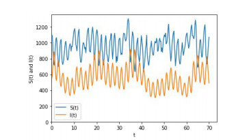
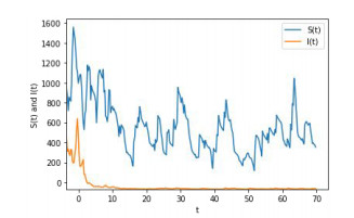
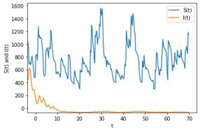
In this paper, we study a nonautonomous stochastic $ SIS $ epidemic model with L$ \acute {e} $vy jumps. We first establish that this model has a unique global positive solution with the positive initial condition. Then, we investigate the condition for extinction of the disease. Moreover, by constructing suitable stochastic Lyapunov function, sufficient conditions for persistence and existence of Nontrivial T-periodic solution of system are obtained. Finally, numerical simulations are also presented to illustrate the main results.
- nonautonomous stochastic $ SIS $ epidemic model,
- L$ \acute {e} $vy jumps,
- Lyapunov function,
- T-periodic solution,
- Extinction and persistence
Citation: Long Lv, Xiao-Juan Yao. Qualitative analysis of a nonautonomous stochastic $ SIS $ epidemic model with L$ \acute {e} $vy jumps[J]. Mathematical Biosciences and Engineering, 2021, 18(2): 1352-1369. doi: 10.3934/mbe.2021071

Related Papers:

Abstract

In this paper, we study a nonautonomous stochastic $ SIS $ epidemic model with L$ \acute {e} $vy jumps. We first establish that this model has a unique global positive solution with the positive initial condition. Then, we investigate the condition for extinction of the disease. Moreover, by constructing suitable stochastic Lyapunov function, sufficient conditions for persistence and existence of Nontrivial T-periodic solution of system are obtained. Finally, numerical simulations are also presented to illustrate the main results.

References

[1]	W. O. Kermack, A. G. McKendrick, A contributions to the mathematical theory of epidemics (Part Ⅰ), Proc. R. Soc. Lond. A., 115 (1927), 700–721.
[2]	H. W. Hethcote, P. Driessche, An $SIS$ epidemic model with variable population size and a delay, J. Math. Biol., 34 (1995), 177–194.
[3]	J. Q. Li, Z. E. Ma, Qualitative analyses of $SIS$ epidemic model with vaccination and varying total population size, Math. Comput. Model., 35 (2002), 1235–1243.
[4]	Y. C. Zhou, H. W. Liu, Satbility of periodic solutions for an $SIS$ model with pulse vaccination, Math. Comput. Model., 38 (2003), 299–308.
[5]	Z. L. Feng, W. Z. Huang, C. Castillo-Chavez, Global behavior of a muli-group $SIS$ epidemic model with age structure, J. Differ. Equ., 218 (2005), 292–324.
[6]	Y. N. Xiao, L. S. Chen, An $SIS$ epidemic with stage structure and a delay, Acta. Math. Appl. Sin., 18 (2002), 607–618.
[7]	A. D'Onofrio, A note on the global behaviour of the network-based $SIS$ epidemic model, Nonlinear. Anal-Real., 9 (2008), 1567–1572.
[8]	F. L. Santos, M. L. Almeida, E. L. Albuquerque, A. Macedo-Filho, M. L. Lyra, U. L. Fulco, Critical properties of the SIS model on the clustered homophilic network, Phys. A, 559 (2020), 125067.
[9]	L. F. Silva, R. N. Costa Filho, A. R. Cunha, A. Macedo-Filho, M. Serva, U. L. Fulco, et al, Critical properties of the SIS model dynamics on the Apollonian network, J. Stat. Mech., 2013, P05003.
[10]	Y. N. Zhao, D. Q. Jiang, D. O'Regan, The extinction and persistence of the stochastic $SIS$ epidemic model with vaccibation, Phys. A., 392 (2013), 4916–4927.
[11]	Y. G. Lin, D. G. Jiang, S. Wang, Stationary distribution of a stochastic $SIS$ epidemic model with vaccination, Phys. A., 394 (2014), 187–197.
[12]	X. B. Zhang, S. Q. Chang, Q. H. Shi, H. F. Huo, Qualitative study of a stochastic $SIS$ epidemic model with vertical transmission, Phys. A., 505 (2018), 805–817.
[13]	X. H. Zhang, D. Q. Jiang, A. Alsaedi, T. Hayat, Stationary distribution of stochastic $SIS$ epidemic model with vaccination under regime switching, Appl. Math. Lett., 59 (2016), 87–93.
[14]	Q. Badshan, G. U. Rahman, R. P. Agarwal, S. Islam, F. JAN, Applications of ergodic theory and dynamical aspects of stochastic hepatitis-c model, Dynam. Syst. Appl., 29 (2020), 139-181.
[15]	R. P. Agarwal, Q. Badshah, G. U. Rahman, S. Islam, Optimal control & dynamical aspects of a stochastic pine wilt disease model, J. Franklin. I., 356 (2019).
[16]	J. H. Bao, X. R. Mao, G. Yin, C. G. Yuan, Competitive Lotka-Volterra population dynamics with jumps, Nonlinear. Anal., 74 (2011), 6601–6616.
[17]	X. B. Zhang, Q. H. Shi, S. H. Ma, H. F. Huo, D. G. Li, Dynamic behavior of a stochastic $SIQS$ epidemic model with L$\acute {e}$vy jumps, Nonlinear. Dynam., 93 (2018), 1481–1493.
[18]	T. Caraballo, A. Settati, M. Fatini, A. Lahrouz, A. Imlahi, Global stability and positive recurrence of a stochastic $SIS$ model with L$\acute {e}$vy noise perturbation, Phys. A., 523 (2019), 677–690.
[19]	M. Naim, F. Lahmidi, A. Namir, Extinction and persistence of a stochastic $SIS$ epidemic model with vertical transmission, specific functional response and L$\acute {e}$vy jumps, Commun. Math. Biol. Neurosci., 15 (2019).
[20]	D. Applebaum, L$\acute {e}$vy processes and stochastic calculus, 2nd edition, Cambridge University Press, 2009.
[21]	J. H. Bao, C. G. Yuan, Stochastic population dynamics driven by L$\acute {e}$vy noise, J. Math. Anal. Appl., 391 (2012), 363–375.
[22]	Y. L. Zhou, S. L. Yuan, D. L. Zhao, Threshold behavior of a stochastic $SIS$ model with L$\acute {e}$vy jumps, Appl. Math. Comput., 275 (2016), 255–267.
[23]	S. Q. Zhang, X. Z. Meng, T. Feng, T. H. Zhang, Dynamics analysis and numerical simulations of a stochastic non-autonomous predator-prey system with impulsive effects, Nonlinear. Anal-Hybri., 26 (2017), 19–37.
[24]	M. Liu, K. Wang, Dynamics of a Leslie-Gower Holling-type $II$ predator-prey system with L$\acute {e}$vy jumps, Nonlinear. Anal., 85 (2013), 204–213.
[25]	C. Liu, M. Liu, Stochastic dynamics in a nonautonomous prey-predator system with impulsive perturbations and L$\acute {e}$vy jumps, Commun. Nonlinear. Sci. Simulat., 2019, 78.
[26]	H. K. Qi, L. D. Liu, X. Z. Meng, Dynamics of a nonautonomous stochastic $SIS$ epidemic model with double epidemic hypothesis, Complexity, 2017, 18.
[27]	W. W. Zhang, X. Z. Meng, Stochastic analysis of a novel nonautonomous periodic $SIRI$ epidemic system with random disturbances, Phys. A., 492 (2018), 1290–1301.
[28]	X. R. Mao, Stochastic differential equations and applications, 2nd edition, Horwood Publishing Limited, 2008.
[29]	B. $\phi$ksendal, A. Sulem, Applied stochastic control of jump diffusions, Springer-Verlag, 2005.
[30]	R. Khasminskii, Stochastic stability of differential equations, Springer-Verlag, 2011.

Reader Comments

Your name:*

Email:*
© 2021 the Author(s), licensee AIMS Press. This is an open access article distributed under the terms of the Creative Commons Attribution License (http://creativecommons.org/licenses/by/4.0)