The quantum statistics mechanism is very powerful for investigating the equilibrium states and the phase transitions in complex spin disorder systems. The spin disorder systems act as an interdisciplinary platform for solving the optimum processes in computer science. In this work, I determined the lower bound of the computational complexity of knapsack problems. I investigated the origin of nontrivial topological structures in these hard problems. It was uncovered that the nontrivial topological structures arise from the contradictory between the three-dimensional character of the lattice and the two-dimensional character of the transfer matrices used in the quantum statistics mechanism. I illustrated a phase diagram for the non-deterministic polynomial (NP) vs polynomial (P) problems, in which a NP-intermediate (NPI) area exists between the NP-complete problems and the P-problems, while the absolute minimum core model is at the border between the NPI and the NP-complete problems. The absolute minimum core model of the knapsack problem cannot collapse directly into the P-problem. Under the guide of the results, one may develop the best algorithms for solving various optimum problems in the shortest time (improved greatly from O(1.3N) to O((1+ε)N) with ε→0 and ε≠1/N) being in subexponential and superpolynomial. This work illuminates the road on various fields of science ranging from physics to biology to finances, and to information technologies.
Citation: Zhidong Zhang. Lower bound of computational complexity of knapsack problems[J]. AIMS Mathematics, 2025, 10(5): 11918-11938. doi: 10.3934/math.2025538
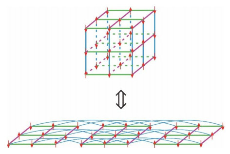
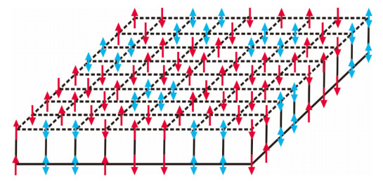
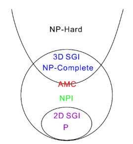
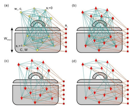
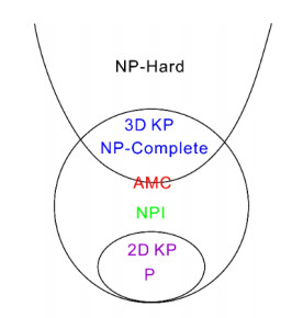
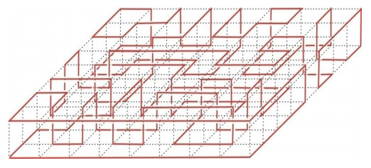
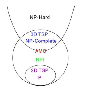
The quantum statistics mechanism is very powerful for investigating the equilibrium states and the phase transitions in complex spin disorder systems. The spin disorder systems act as an interdisciplinary platform for solving the optimum processes in computer science. In this work, I determined the lower bound of the computational complexity of knapsack problems. I investigated the origin of nontrivial topological structures in these hard problems. It was uncovered that the nontrivial topological structures arise from the contradictory between the three-dimensional character of the lattice and the two-dimensional character of the transfer matrices used in the quantum statistics mechanism. I illustrated a phase diagram for the non-deterministic polynomial (NP) vs polynomial (P) problems, in which a NP-intermediate (NPI) area exists between the NP-complete problems and the P-problems, while the absolute minimum core model is at the border between the NPI and the NP-complete problems. The absolute minimum core model of the knapsack problem cannot collapse directly into the P-problem. Under the guide of the results, one may develop the best algorithms for solving various optimum problems in the shortest time (improved greatly from O(1.3N) to O((1+ε)N) with ε→0 and ε≠1/N) being in subexponential and superpolynomial. This work illuminates the road on various fields of science ranging from physics to biology to finances, and to information technologies.

| [1] | K. Huang, Statistical mechanics, New York: Wiley, 2008. |
| [2] |
C. P. Bachas, Computer-intractability of the frustration model of a spin glass, J. Phys. A: Math. Gen., 17 (1984), L709. https://doi.org/10.1088/0305-4470/17/13/006 doi: 10.1088/0305-4470/17/13/006

|
| [3] |
F. Barahona, On the computational complexity of Ising spin glass models, J. Phys. A: Math. Gen., 15 (1982), 3241. https://doi.org/10.1088/0305-4470/15/10/028 doi: 10.1088/0305-4470/15/10/028
|
| [4] |
S. F. Edwards, P. W. Anderson, Theory of spin glasses, J. Phys. F: Met. Phys., 5 (1975), 965–974. https://doi.org/10.1088/0305-4608/5/5/017 doi: 10.1088/0305-4608/5/5/017
|
| [5] |
S. Istrail, Statistical mechanics, three-dimensionality and NP-completeness: I. Universality of intracatability for the partition function of the Ising model across non-planar surfaces (extended abstract), Proceedings of the Thirty-Second Annual ACM Symposium on Theory of Computing, 2000, 87–96. https://doi.org/10.1145/335305.335316 doi: 10.1145/335305.335316
|
| [6] | D. L. Stein, C. M. Newman, Spin glasses and complexity, Princeton University Press, 2013. |
| [7] |
E. Ising, Beitrag zur theorie des ferromagnetismus, Z. Phys., 31 (1925), 253–258. https://doi.org/10.1007/BF02980577 doi: 10.1007/BF02980577
|
| [8] |
L. Onsager, Crystal statistics I: a two-dimensional model with an order-disorder transition, Phys. Rev., 65 (1944), 117–149. https://doi.org/10.1103/PhysRev.65.117 doi: 10.1103/PhysRev.65.117
|
| [9] |
Z. D. Zhang, Conjectures on the exact solution of three-dimensional (3D) simple orthorhombic Ising lattices, Phil. Mag., 87 (2007), 5309–5419. https://doi.org/10.1080/14786430701646325 doi: 10.1080/14786430701646325
|
| [10] | M. Garey, D. S. Johnson, Computers and intractability, A guide to the Theory of NP-completeness, W. H. Freeman and Company, San Francisco, 1979. |
| [11] | C. H. Papadimitriou, Computational complexity, Addison-Wesley, 1994. |
| [12] |
S. Cook, The complexity of theorem-proving procedures, Proceedings of the Third Annual ACM Symposium on Theory of Computing, 1971,151–158. https://doi.org/10.1145/800157.805047 doi: 10.1145/800157.805047
|
| [13] | L. A. Levin, Universal sequential search problems, Probl. Inform. Transm., 9 (1973), 265–266. |
| [14] |
Z. D. Zhang, Computational complexity of spin-glass three-dimensional (3D) Ising model, J. Mater. Sci. Tech., 44 (2020), 116–120. https://doi.org/10.1016/j.jmst.2019.12.009 doi: 10.1016/j.jmst.2019.12.009
|
| [15] |
Z. D. Zhang, Mapping between spin-glass three-dimensional (3D) Ising model and Boolean satisfiability problem, Mathematics, 11 (2023), 237. https://doi.org/10.3390/math11010237 doi: 10.3390/math11010237
|
| [16] | T. Dantzig, Numbers: the language of science, London: George Allen & Unwin, Ltd., 1930. |
| [17] |
G. B. Mathews, On the partition of numbers, Proc. London Math. Soc., 28 (1897), 486–490. https://doi.org/10.1112/plms/s1-28.1.486 doi: 10.1112/plms/s1-28.1.486
|
| [18] |
S. Martello, D. Pisinger, P. Toth, New trends in exact algorithms for the 0-1 knapsack problem, Eur. J. Oper. Res., 123 (2000), 325–332. https://doi.org/10.1016/S0377-2217(99)00260-X doi: 10.1016/S0377-2217(99)00260-X
|
| [19] | D. Pisinger, Where are the hard knapsack problems? Comput. Oper. Res., 32 (2005), 2271–2284. https://doi.org/10.1016/j.cor.2004.03.002 |
| [20] |
D. Fayard, G. Plateau, Resolution of the 0-1 knapsack problem: comparison of methods, Math. Program., 8 (1975), 272–307. https://doi.org/10.1007/BF01580448 doi: 10.1007/BF01580448
|
| [21] |
S. Sahni, Approximate algorithms for the 0-1 knapsack problem, J. ACM, 22 (1975), 115–124. https://doi.org/10.1145/321864.321873 doi: 10.1145/321864.321873
|
| [22] |
S. Al-Shihabi, A novel core-based optimization framework for binary integer programs- the multidemand multidimesional knapsack problem as a test problem, Oper. Res. Perspect., 8 (2021), 100182. https://doi.org/10.1016/j.orp.2021.100182 doi: 10.1016/j.orp.2021.100182
|
| [23] |
D. E. Armstrong, S. H. Jacobson, Data-independent neighborhood functions and strict local optima, Discrete Appl. Math., 146 (2005), 233–243. https://doi.org/10.1016/j.dam.2004.09.007 doi: 10.1016/j.dam.2004.09.007
|
| [24] |
D. S. Johnson, Approximation algorithms for combinatorial problems, J. Comput. Syst. Sci., 9 (1974), 256–278. https://doi.org/10.1016/S0022-0000(74)80044-9 doi: 10.1016/S0022-0000(74)80044-9
|
| [25] |
P. Toth, Optimization engineering techniques for the exact solution of NP-hard combinatorial optimization problems, Eur. J. Oper. Res., 125 (2000), 222–238. https://doi.org/10.1016/S0377-2217(99)00453-1 doi: 10.1016/S0377-2217(99)00453-1
|
| [26] |
G. Venkataraman, G. Athithan, Spin glass, the travelling salesman problem, neural networks and all that, Pramana-J. Phys., 36 (1991), 1–77. https://doi.org/10.1007/BF02846491 doi: 10.1007/BF02846491
|
| [27] |
Z. D. Zhang, O. Suzuki, N. H. March, Clifford algebra approach of 3D Ising model, Adv. Appl. Clifford Algebras, 29 (2019), 12. https://doi.org/10.1007/s00006-018-0923-2 doi: 10.1007/s00006-018-0923-2
|
| [28] |
O. Suzuki, Z. D. Zhang, A method of Riemann-Hilbert problem for Zhang's conjecture 1 in a ferromagnetic 3D Ising model: trivialization of topological structure, Mathematics, 9 (2021), 776. https://doi.org/10.3390/math9070776 doi: 10.3390/math9070776
|
| [29] |
B. C. Li, W. Wang, Exploration of dynamic phase transition of 3D Ising model with a new long-range interaction by using the Monte Carlo method, Chin. J. Phys., 90 (2024), 15–30. https://doi.org/10.1016/j.cjph.2024.05.021 doi: 10.1016/j.cjph.2024.05.021
|
| [30] |
K. Ghosh, C. J. Lobb, R. L. Greene, Critical phenomena in the double-exchange ferromagnet La0.7Sr0.3MnO3, Phys. Rev. Lett., 81 (1998), 4740–4743. https://doi.org/10.1103/PhysRevLett.81.4740 doi: 10.1103/PhysRevLett.81.4740
|
| [31] |
J. T. Ho, J. D. Litster, Magnetic equation of state of CrBr3 near the critical point, Phys. Rev. Lett., 22 (1969), 603–606. https://doi.org/10.1103/PhysRevLett.22.603 doi: 10.1103/PhysRevLett.22.603
|
| [32] |
Y. Liu, V. N. Ivanovski, C. Petrovic, Critical behavior of the van der Waals bonded ferromagnet Fe3-xGeTe2, Phys. Rev. B, 96 (2017), 144429. https://doi.org/10.1103/PhysRevB.96.144429 doi: 10.1103/PhysRevB.96.144429
|
| [33] |
F. X. Liu, L. M. Duan, Computational characteristics of the random-field Ising model with long-range interaction, Phys. Rev. A, 108 (2023), 012415. https://doi.org/10.1103/PhysRevA.108.012415 doi: 10.1103/PhysRevA.108.012415
|
| [34] |
S. Nagy, R. Paredes, J. M. Dudek, L. Dueñas-Osorio, M. Y. Vardi, Ising model partition-function computation as a weighted counting problem, Phys. Rev. E, 109 (2024), 055301. https://doi.org/10.1103/PhysRevE.109.055301 doi: 10.1103/PhysRevE.109.055301
|
| [35] |
H. J. Xu, S. Dasgupta, A. Pothen, A. Banerjee, Dynamic asset allocation with expected shortfall via quantum annealing, Entropy, 25 (2023), 541. https://doi.org/10.3390/e25030541 doi: 10.3390/e25030541
|
| [36] |
R. Ladner, On the structure of polynomial time reducibility, J. ACM, 22 (1975), 155–171. https://doi.org/10.1145/321864.321877 doi: 10.1145/321864.321877
|
| [37] |
P. Jonsson, V. Lagerkvist, G. Nordh, Constructing NP-intermediate problems by blowing holes with parameters of various properties, Theor. Comput. Sci., 581 (2015), 67–82. https://doi.org/10.1016/j.tcs.2015.03.009 doi: 10.1016/j.tcs.2015.03.009
|
| [38] |
R. Bellman, A Markovian decision process, J. Math. Mech., 6 (1957), 679–684. https://doi.org/10.1512/iumj.1957.6.56038 doi: 10.1512/iumj.1957.6.56038
|
| [39] |
O. Kyriienko, H. Sigurdsson, T. C. H. Liew, Probabilistic solving of NP-hard problems with bistable nonlinear optical networks, Phys. Rev. B, 99 (2019), 195301. https://doi.org/10.1103/PhysRevB.99.195301 doi: 10.1103/PhysRevB.99.195301
|
| [40] |
G. B. Dantzig, Discrete-variable extremum problems, Oper. Res., 5 (1957), 161–306. https://doi.org/10.1287/opre.5.2.266 doi: 10.1287/opre.5.2.266
|
| [41] |
R. Bellman, Letter to the Editor–Comment on Dantzig's paper on discrete-variable extremum problems, Oper. Res., 5 (1957), 613–738. https://doi.org/10.1287/opre.5.5.723 doi: 10.1287/opre.5.5.723
|
| [42] |
V. Cacchiani, M. Iori, A. Locatelli, S. Martello, Knapsack problems–an overview of recent advances. Part I: single knapsack problems, Comput. Oper. Res., 143 (2022), 105692. https://doi.org/10.1016/j.cor.2021.105692 doi: 10.1016/j.cor.2021.105692
|
| [43] | V. Cacchiani, M. Iori, A. Locatelli, S. Martello, Knapsack problems–an overview of recent advances. Part Ⅱ: Multiple, multidimensional, and quadratic knapsack problems, Comput. Oper. Res., 143 (2022), 105693. https://doi.org/10.1016/j.cor.2021.105693 |
| [44] | H. Kellerer, U. Pferschy, D. Pisinger, Knapsack problems, Springer-Verlag, 2004. https://doi.org/10.1007/978-3-540-24777-7 |
| [45] | H. Nishimori, Statistical physics of spin glasses and information processing: an introduction, Oxford University Press, 2001. |
| [46] |
S. Kirkpatrick, D. Sherrington, Infinite-ranged models of spin-glasses, Phys. Rev. B, 17 (1978), 4384–4403. https://doi.org/10.1103/PhysRevB.17.4384 doi: 10.1103/PhysRevB.17.4384
|
| [47] |
D. Sherrington, S. Kirkpatrick, Solvable model of a spin-glass, Phys. Rev. Lett., 35 (1975), 1792–1796. https://doi.org/10.1103/PhysRevLett.35.1792 doi: 10.1103/PhysRevLett.35.1792
|
| [48] |
S. Boccaletti, V. Latora, Y. Moreno, M. Chavez, D. U. Hwang, Complex networks: structure and dynamics, Phys. Rep., 424 (2006), 175–308. https://doi.org/10.1016/j.physrep.2005.10.009 doi: 10.1016/j.physrep.2005.10.009
|
| [49] |
G. E. Hinton, R. R. Salakhutdinov, Reducing the dimensionality of data with neural networks, Science, 313 (2006), 504–507. https://doi.org/10.1126/science.1127647 doi: 10.1126/science.1127647
|
| [50] | M. K. Kwan, Graphic programming using odd or even points, Chin. Math., 1(1962), 273–277. |
| [51] |
U. U. Haus, K. Niermann, K. Truemper, R. Weismantel, Logic integer programming models for signaling networks, J. Comput. Biol., 16 (2009), 725–743. https://doi.org/10.1089/cmb.2008.0163 doi: 10.1089/cmb.2008.0163
|
| [52] |
D. Bertsimas, R. Demir, An approximate dynamic programming approach to multidimensional Knapsack problems, Manag. Sci., 48 (2002), 453–590. https://doi.org/10.1287/mnsc.48.4.550.208 doi: 10.1287/mnsc.48.4.550.208
|
| [53] | G. J. Woeginger, When does a dynamic programming formulation guarantee the existence of a fully polynomial time approximation scheme (FPTAS)? J. Comput., 12 (2000), 1–82. https://doi.org/10.1287/ijoc.12.1.57.11901 |
| [54] |
E. Balas, N. Simonetti, Linear time dynamic-programming algorithms for new classes of restricted TSPs: a computational study, J. Comput., 13 (2001), 1–94. https://doi.org/10.1287/ijoc.13.1.56.9748 doi: 10.1287/ijoc.13.1.56.9748
|
| [55] |
A. A. Melkman, T. Akutsu, An improved satisfiability algorithm for nested canalyzing functions and its application to determining a singleton attractor of a Boolean network, J. Comput. Biol., 20 (2013), 958–969. https://doi.org/10.1089/cmb.2013.0060 doi: 10.1089/cmb.2013.0060
|
| [56] |
P. C. Chu, J. E. Beasley, A genetic algorithm for the multidimensional Knapsack problem, J. Heuristics, 4 (1998), 63–86. https://doi.org/10.1023/A:1009642405419 doi: 10.1023/A:1009642405419
|
| [57] |
A. K. Hartmann, Ground-state behavior of the three-dimensional ±J random-bond Ising model, Phys. Rev. B, 59 (1999), 3617. https://doi.org/10.1103/PhysRevB.59.3617 doi: 10.1103/PhysRevB.59.3617
|
| [58] |
L. V. Snyder, M. S. Daskin, A random-key genetic algorithm for the generalized traveling salesman problem, Eur. J. Oper. Res., 174 (2006), 38–53. https://doi.org/10.1016/j.ejor.2004.09.057 doi: 10.1016/j.ejor.2004.09.057
|
| [59] |
P. Larranaga, C. M. H. Kuijpers, R. H. Murga, I. Inza, S. Dizdarevic, Genetic algorithms for the travelling salesman problem: a review of representations and operators, Artif. Intell. Rev., 13 (1999), 129–170. https://doi.org/10.1023/A:1006529012972 doi: 10.1023/A:1006529012972
|
Figures(7)

Zhidong Zhang. Lower bound of computational complexity of knapsack problems[J]. AIMS Mathematics, 2025, 10(5): 11918-11938. doi: 10.3934/math.2025538


 DownLoad: