Noble-Abel gas diffusion at convex corners of the two-dimensional compressible magnetohydrodynamic system

Fei Zhu; Fei Zhu

doi:10.3934/math.20241156

AIMS Mathematics

2024, Volume 9, Issue 9: 23786-23811. doi: 10.3934/math.20241156

Previous Article Next Article

Research article

Noble-Abel gas diffusion at convex corners of the two-dimensional compressible magnetohydrodynamic system

Fei Zhu ^,

College of Mathematics and System Sciences, Xinjiang University, Urumqi, 830017, China

Received: 11 June 2024 Revised: 30 July 2024 Accepted: 05 August 2024 Published: 09 August 2024
MSC : 35A01, 76N25

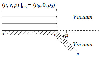
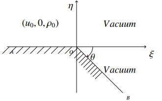
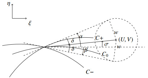
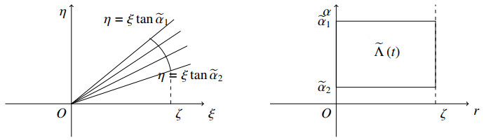
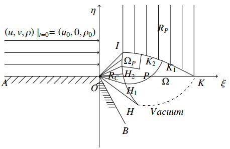
In this paper, we study the expansion of Noble-Abel gas into a vacuum around the convex corner of the two-dimensional compressible magnetohydrodynamic system. We reduce this problem to the interaction of a centered simple wave emanating from the convex corner with a backward planar simple wave. Mathematically, this is a Goursat problem. By using the method of characteristic decomposition and construction of invariant regions, combining $ C^{0} $ and $ C^{1} $ estimation as well as hyperbolicity estimation, we obtain the existence of a global classical solution by extending the local classical solution.
- gas diffusion,
- convex corner,
- compressible magnetohydrodynamic system,
- Noble-Able gas,
- goursat problem
Citation: Fei Zhu. Noble-Abel gas diffusion at convex corners of the two-dimensional compressible magnetohydrodynamic system[J]. AIMS Mathematics, 2024, 9(9): 23786-23811. doi: 10.3934/math.20241156

Related Papers:

Abstract

In this paper, we study the expansion of Noble-Abel gas into a vacuum around the convex corner of the two-dimensional compressible magnetohydrodynamic system. We reduce this problem to the interaction of a centered simple wave emanating from the convex corner with a backward planar simple wave. Mathematically, this is a Goursat problem. By using the method of characteristic decomposition and construction of invariant regions, combining $ C^{0} $ and $ C^{1} $ estimation as well as hyperbolicity estimation, we obtain the existence of a global classical solution by extending the local classical solution.

References

[1]	B. Ducomet, E. Feireisl, The equations of magnetohydrodynamics: On the interaction between matter and radiation in the evolution of gaseous stars, Commun. Math. Phys., 266 (2006), 595–629. https://doi.org/10.1007/s00220-006-0052-y doi: 10.1007/s00220-006-0052-y
[2]	L. D. Landau, E. M. Lifshitz, GElectrodynamics of continuous media, Pergamon Press Oxford, 1946.
[3]	M. A. Liberman, A. L. Velikovich, A. S. Dobroslavski, Physics of shock waves in gases and plasmas, Springer, 1986.
[4]	T. Li, T. Qin, Physics and partial differential equations, Higher Education Press, 2005.
[5]	R. Courant, K. O. Friedrichs, Supersonic Flow and Shock Waves, Interscience Publishers, 1948.
[6]	W. C. Sheng, S. K. You, Interaction of a centered simple wave and a planar rarefaction wave of the two-dimensional Euler equations for pseudo-steady compressible flow, J. Math. Pure Appl., 114 (2018), 29–50. https://doi.org/10.1016/j.matpur.2017.07.019 doi: 10.1016/j.matpur.2017.07.019
[7]	W. C. Sheng, A. D. Yao, Centered simple waves for the two-dimensional pseudo-steady isothermal flow around a convex corner, Appl. Math. Mech., 40 (2019), 705–718. https://doi.org/10.1007/s10483-019-2475-6 doi: 10.1007/s10483-019-2475-6
[8]	J. J. Chen, Z. M. Shen, G. Yin, The expansion of a non-ideal gas around a sharp corner for 2-D compressible Euler system, Math. Method. Appl. Sci., 46 (2023), 2023–2041.
[9]	S. R. Li, W. C. Sheng, Two-dimensional Riemann problem of the Euler equations to the Van der Waals gas around a sharp corner, Stud. Appl. Math., 152 (2023). https://doi.org/10.1111/sapm.12658
[10]	T. Zhang, Y. X. Zheng, Conjecture on the structure of solutions of the Riemann problem for two-dimensional gas dynamics systems, SIAM J. Math. Anal., 21 (1990), 593–630. https://doi.org/10.1137/0521032 doi: 10.1137/0521032
[11]	X. Chen, Y. X. Zheng, The interaction of rarefaction waves of the two-dimensional Euler equations, Indiana U. Math. J., 59 (2010), 231–256. https://doi.org/10.1512/iumj.2010.59.3752 doi: 10.1512/iumj.2010.59.3752
[12]	J. Q. Li, Z. C. Yang, Y. X. Zheng, Characteristic decompositions and interactions of rarefaction waves of 2-D Euler equations, J. Differ. Equations, 250 (2011), 782–798. https://doi.org/10.1016/j.jde.2010.07.009 doi: 10.1016/j.jde.2010.07.009
[13]	J. J. Chen, G. Yin, The expansion of supersonic flows into a vacuum through a convex duct with limited length, Z. Angew. Math. Phys., 69 (2018), 1–13. https://doi.org/10.1007/s00033-018-0994-x doi: 10.1007/s00033-018-0994-x
[14]	J. Q. Li, Y. X. Zheng, Interaction of rarefaction waves of the two-dimensional self-similar Euler equations, Arch. Ration. Mech. An., 193 (2009), 623–657. https://doi.org/10.1007/s00205-008-0140-6 doi: 10.1007/s00205-008-0140-6
[15]	T. Zhang, Z. H. Dai, Existence of a global smooth solution for a degenerate Goursat problem of gas dynamics, Arch. Ration. Mech. An., 155 (2000), 277–298. https://doi.org/10.1007/s002050000113 doi: 10.1007/s002050000113
[16]	Y. B. Hu, J. Q. Li, W. C. Sheng, Degenerate Goursat-type boundary value problems arising from the study of two-dimensional isothermal Euler equations, Z. Angew. Math. Phys., 63 (2012), 1021–1046. https://doi.org/10.1007/s00033-012-0203-2 doi: 10.1007/s00033-012-0203-2
[17]	Y. B. Hu, G. D. Wang, The interaction of rarefaction waves of a two-dimensional nonlinear wave system, Nonlinear Anal.-Real, 22 (2015), 1–15. https://doi.org/10.1016/j.nonrwa.2014.07.009 doi: 10.1016/j.nonrwa.2014.07.009
[18]	G. Lai, On the expansion of a wedge of van der Waals gas into a vacuum, J. Differ. Equations, 259 (2015), 1181–1202. https://doi.org/10.1016/j.jde.2015.02.039 doi: 10.1016/j.jde.2015.02.039
[19]	J. Q. Li, On the two-dimensional gas expansion for compressible Euler equations, SIAM J. Appl. Math., 62 (2002), 831–852. https://doi.org/10.1137/S0036139900361349 doi: 10.1137/S0036139900361349
[20]	G. Lai, Interactions of composite waves of the two-dimensional full Euler equations for van der Waals gases, SIAM J. Math. Anal., 50 (2018), 3535–3597. https://doi.org/10.1137/17M1144660 doi: 10.1137/17M1144660
[21]	L. P. Luan, J. J. Chen, J. L. Liu, Two dimensional relativistic Euler equations in a convex duct, J. Math. Anal. Appl., 461 (2018), 1084–1099. https://doi.org/10.1016/j.jmaa.2018.01.033 doi: 10.1016/j.jmaa.2018.01.033
[22]	F. B. Li, W. Xiao, Interaction of four rarefaction waves in the bi-symmetric class of the pressure-gradient system, J. Differ. Equations, 252 (2012), 3920–3952. https://doi.org/10.1016/j.jde.2011.11.010 doi: 10.1016/j.jde.2011.11.010
[23]	M. Zafar, V. D. Sharma, Expansion of a wedge of non-ideal gas into vacuum, Nonlinear Anal.-Real, 31 (2016), 580–592. https://doi.org/10.1016/j.nonrwa.2016.03.006 doi: 10.1016/j.nonrwa.2016.03.006
[24]	W. X. Zhao, The expansion of gas from a wedge with small angle into a vacuum, Commun. Pure Appl. Anal., 12 (2013). https://doi.org/10.3934/cpaa.2013.12.2319
[25]	G. Lai, On the expansion of a wedge of Van der Waals gas into a vacuum Ⅱ, J. Differ. Equations, 260 (2016), 3538–3575. https://doi.org/10.1016/j.jde.2015.10.048 doi: 10.1016/j.jde.2015.10.048
[26]	J. J. Chen, G. Yin, S. K. You, Expansion of gas by turning a sharp corner into vacuum for 2-D pseudo-steady compressible magnetohydrodynamics system, Nonlinear Anal.-Real, 52 (2020), 102955. https://doi.org/10.1016/j.nonrwa.2019.06.005 doi: 10.1016/j.nonrwa.2019.06.005
[27]	J. Q. Li, T. Zhang, Y. X. Zheng, Simple waves and a characteristic decomposition of the two dimensional compressible Euler equations, Commun. Math. Phys., 267 (2006), 1–12. https://doi.org/10.1007/s00220-006-0033-1 doi: 10.1007/s00220-006-0033-1
[28]	T. Li, W. C. Yu, Boundary value problems of quasilinear hyperbolic system, Duke Univers. Math. Ser., vol. V, Mathematics Dept., 1985.
[29]	T. G. Cowling, Magnetoydrodynamics, Interscience, 1957.

Reader Comments

Your name:*

Email:*
© 2024 the Author(s), licensee AIMS Press. This is an open access article distributed under the terms of the Creative Commons Attribution License (http://creativecommons.org/licenses/by/4.0)