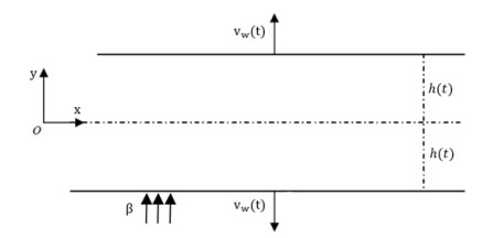
We introduce this work by studying the non-Newtonian fluids, which have huge applications in different science fields. We decided to concentrate on taking the time-dependent Casson fluid, which is non-Newtonian, compressed between two flat plates. in fractional form and the magnetohydrodynamic and Darcian flow effects in consideration using the semi-analytical iterative method created by Temimi and Ansari, known as TAM, this method is carefully selected to be suitable for studying the Navier-Stokes model in the modified form to express the studied case mathematically. To simplify the partial differential equations of the system to the nonlinear ordinary differential equation of order four the similarity transformations suggested by Wang (1976) are used. The TAM approach demonstrates a high degree of accuracy, efficiency, and convergence when applied to the resolution of both linear and nonlinear problems, and the results in this article are used to study the effect of the related factors like squeeze number Sq, Casson parameterβ, magnetohydrodynamic parameter Mg and permeability constant Mp and examining the skin friction coefficient effect. The velocity profile is studied numerically, which is tabulated and graphically represented to show and confirm the theoretical study. We can conclude that the success of the proposed method in studying time-dependent Casson fluid, which is non-Newtonian, compressed between two flat plates provides opportunities for additional study and advancements in fluid mechanics using the techniques.
Citation: Amal Al-Hanaya, Munirah Alotaibi, Mohammed Shqair, Ahmed Eissa Hagag. MHD effects on Casson fluid flow squeezing between parallel plates[J]. AIMS Mathematics, 2023, 8(12): 29440-29452. doi: 10.3934/math.20231507
We introduce this work by studying the non-Newtonian fluids, which have huge applications in different science fields. We decided to concentrate on taking the time-dependent Casson fluid, which is non-Newtonian, compressed between two flat plates. in fractional form and the magnetohydrodynamic and Darcian flow effects in consideration using the semi-analytical iterative method created by Temimi and Ansari, known as TAM, this method is carefully selected to be suitable for studying the Navier-Stokes model in the modified form to express the studied case mathematically. To simplify the partial differential equations of the system to the nonlinear ordinary differential equation of order four the similarity transformations suggested by Wang (1976) are used. The TAM approach demonstrates a high degree of accuracy, efficiency, and convergence when applied to the resolution of both linear and nonlinear problems, and the results in this article are used to study the effect of the related factors like squeeze number Sq, Casson parameterβ, magnetohydrodynamic parameter Mg and permeability constant Mp and examining the skin friction coefficient effect. The velocity profile is studied numerically, which is tabulated and graphically represented to show and confirm the theoretical study. We can conclude that the success of the proposed method in studying time-dependent Casson fluid, which is non-Newtonian, compressed between two flat plates provides opportunities for additional study and advancements in fluid mechanics using the techniques.

| [1] |
R. L. Batra, B. Jena, Flow of a Casson fluid in a slightly curved tube, Int. J. Eng. Sci. , 29 (1991), 1245–1258. https://doi.org/10.1016/0020-7225(91)90028-2 doi: 10.1016/0020-7225(91)90028-2

|
| [2] |
M. Mustafa, T. Hayat, I. Pop, A. Aziz, Unsteady boundary layer flow of a Casson fluid due to an impulsively started moving flat plate, Heat Transf. Asian Res. , 40 (2011), 563–576. https://doi.org/10.1002/htj.20358 doi: 10.1002/htj.20358
|
| [3] |
W. Ibrahim, T. Anbessa, Three-dimensional MHD mixed convection flow of Casson nanofluid with hall and ion slip effects, Math. Prob. Eng. , 2020 (2020), 8656147. https://doi.org/10.1155/2020/8656147 doi: 10.1155/2020/8656147
|
| [4] |
B. Manvi, S. B. Kerur, J. V. Tawade, J. J. Nieto, S. N. Sankeshwari, H. Ahmad, et al., MHD Casson nanofluid boundary layer flow in presence of radiation and non-uniform heat source/sink, Math. Model. Control, 3 (2023), 152–167. http://dx.doi.org/10.3934/mmc.2023014 doi: 10.3934/mmc.2023014
|
| [5] | R. Moreau, Magnetohydrodynamics, Berlin: Springer, 1990. |
| [6] |
K. Krupalakshmi, B. J. Gireesha, B. Mahanthesh, R. Gorla, Influence of nonlinear thermal radiation and Magnetic field on upper-convected Maxwell fluid flow due to a convectively heated stretching sheet in the presence of dust particles, Commun. Numer. Anal. , 2016 (2016), 57–73. http://dx.doi.org/10.5899/2016/cna-00254 doi: 10.5899/2016/cna-00254
|
| [7] |
S. Das, S. Sarkar, R. N. Jana, Entropy generation analysis of MHD slip flow of non-Newtonian Cu-Casson nanofluid in a porous microchannel filled with saturated porous medium considering thermal radiation, J. Nanofluids, 7 (2018), 1217–1232. https://doi.org/10.1166/jon.2018.1530 doi: 10.1166/jon.2018.1530
|
| [8] |
M. M. Rashidi, Z. Yang, M. M. Bhatti, M. A. Abbas, Heat and mass transfer analysis on MHD blood flow of Casson fluid model due to peristaltic wave, Thermal Sci. , 22 (2018), 2439–2448. https://doi.org/10.2298/TSCI160102287R doi: 10.2298/TSCI160102287R
|
| [9] |
A. Hamarsheh, F. A. Alwawi, H. T. Alkasasbeh, A. M. Rashad, R. Idris, Heat transfer improvement in MHD natural convection flow of graphite oxide/carbon nanotubes-methanol based casson nanofluids past a horizontal circular cylinder, Processes, 8 (2020), 1444. https://doi.org/10.3390/pr8111444 doi: 10.3390/pr8111444
|
| [10] |
E. El-Zahar, A. E. N. Mahdy, A. M. Rashad, W. Saad, L. F. Seddek, Unsteady MHD mixed convection flow of Non-Newtonian Casson hybrid nanofluid in the stagnation zone of sphere spinning impulsively, Fluids, 6 (2021), 197. https://doi.org/10.3390/fluids6060197 doi: 10.3390/fluids6060197
|
| [11] |
J. Jackson, A study of squeezing flow, Appl. Sci. Res. , 11 (1963), 148–152. https://doi.org/10.1007/BF03184719 doi: 10.1007/BF03184719
|
| [12] |
W. Wolfe, Squeeze film pressures, Appl. Sci. Res. , 14 (1965), 77–90. https://doi.org/10.1007/BF00382232 doi: 10.1007/BF00382232
|
| [13] |
M. Ramzan, N. Shaheen, J. D. Chung, S. Kadry, Y. M. Chu, F. Howari, Impact of Newtonian heating and Fourier and Fick's laws on a magnetohydrodynamic dusty Casson nanofluid flow with variable heat source/sink over a stretching cylinder, Sci. Rep. , 11 (2021), 2357. https://doi.org/10.1038/s41598-021-81747-x doi: 10.1038/s41598-021-81747-x
|
| [14] |
Y. M. Chu, N. A. Shah, H. Ahmad, J. D. Chung, S. M. Khaled, A comparative study of semi-analytical methods for solving fractional-order Cauchy reaction-diffusion equation, Fractals, 29 (2021), 2150143. https://doi.org/10.1142/S0218348X21501437 doi: 10.1142/S0218348X21501437
|
| [15] |
N. Ahmed, U. Khan, S. I. Khan, S. Bano, S. T. Mohyud-Din, Effects on magnetic field in squeezing flow of a Casson fluid between parallel plates, J. King Saud Uni. Sci. , 29 (2017), 119–125. https://doi.org/10.1016/j.jksus.2015.03.006 doi: 10.1016/j.jksus.2015.03.006
|
| [16] |
A. Al-Saif, A. Jasim, A novel algorithm for studying the effects of squeezing flow of a Casson Fluid between parallel plates on magnetic field, J. Appl. Math. , 2019 (2019), 3679373. https://doi.org/10.1155/2019/3679373 doi: 10.1155/2019/3679373
|
| [17] | N. Noor, S. Shafie, M. Admon, MHD squeezing flow of Casson nanofluid with chemical reaction, thermal radiation and heat generation/absorption, J. Adv. Res. Fluid Mech. Thermal Sci. , 68 (2020), 94–111. |
| [18] |
B. Divya, G. Manjunatha, C. Rajashekhar, H. Vaidya, K. V. Prasad, Analysis of temperature dependent properties of a peristaltic MHD flow in a non-uniform channel: A Casson fluid model, Ain Shams Eng. J. , 12 (2021), 2181–2191. https://doi.org/10.1016/j.asej.2020.11.010 doi: 10.1016/j.asej.2020.11.010
|
| [19] |
S. Li, K. Raghunath, A. Alfaleh, F. Ali, A. Zaib, M. I. Khan, et al., Effects of activation energy and chemical reaction on unsteady MHD dissipative Darcy-Forchheimer squeezed flow of Casson fluid over horizontal channel, Sci. Rep. , 13 (2023), 2666. https://doi.org/10.1038/s41598-023-29702-w doi: 10.1038/s41598-023-29702-w
|
| [20] | S. Samko, Fractional integrals and derivatives, Theory Appl. , 1993. |
| [21] |
V. Tarasov, S. Tarasova, Fractional derivatives and integrals: What are they needed for? Mathematics, 8 (2020), 164. https://doi.org/10.3390/math8020164 doi: 10.3390/math8020164
|
| [22] |
M. Saqib, I. Khan, S. Shafie, Generalized magnetic blood flow in a cylindrical tube with magnetite dusty particles, J. Magn. Magnetic Mate., 484 (2019), 490–496. https://doi.org/10.1016/j.jmmm.2019.03.032 doi: 10.1016/j.jmmm.2019.03.032
|
| [23] |
V. Kulish, J. Lage, Application of fractional calculus to fluid mechanics, J. Fluids Eng., 124 (2002), 803–806. https://doi.org/10.1115/1.1478062 doi: 10.1115/1.1478062
|
| [24] |
H. Waqas, M. J. Hasan, A. H. Majeed, D. Liu, Taseer Muhammad, Hydrothermal characteristics, entropy and kinetic energy investigation in a sinusoidal cavity for variable wavelengths and solid volume fraction using Cu-water nanofluid, J. Mol. Liq., 389 (2023), 122911. https://doi.org/10.1016/j.molliq.2023.122911 doi: 10.1016/j.molliq.2023.122911
|
| [25] |
S. Rashid, Z. Hammouch, R. Ashraf, Y. M. Chu, New computation of unified bounds via a more general fractional operator using generalized Mittag-Leffler function in the kernel, Comput. Model. Eng. Sci., 126 (2021), 359–378. http://dx.doi.org/10.32604/cmes.2021.011782 doi: 10.32604/cmes.2021.011782
|
| [26] |
H. Waqas, U. Farooq, D. Liu, M. Alghamdi, S. Noreen, T. Muhammad, Numerical investigation of nanofluid flow with gold and silver nanoparticles injected inside a stenotic artery, Mater. Design, 223 (2022), 111130. https://doi.org/10.1016/j.matdes.2022.111130 doi: 10.1016/j.matdes.2022.111130
|
| [27] |
L. Debnath, Recent applications of fractional calculus to science and engineering, Int. J. Math. Mathematical Sci., 2003 (2003), 753601. https://doi.org/10.1155/S0161171203301486 doi: 10.1155/S0161171203301486
|
| [28] |
I. Tejado, E. Pérez, D. Valério, Fractional calculus in economic growth modelling of the group of seven, Fract. Cal. Appl. Anal., 22 (2019), 139–157. https://doi.org/10.1515/fca-2019-0009 doi: 10.1515/fca-2019-0009
|
| [29] |
A. Ali, S. U. Haq, S. I. Ali Shah, I. Khan, A. S. Aljohani, S. U. Jan, et al., Heat transfer analysis of generalized nanofluid with MHD and ramped wall temperature using Caputo-Fabrizio derivative approach, Math. Prob. Eng., 2023 (2023), 8834891. https://doi.org/10.1155/2023/8834891 doi: 10.1155/2023/8834891
|
| [30] |
R. Reyaz, Y. J. Lim, A. Q. Mohamad, M. Saqib, S. Shafie, Caputo fractional MHD Casson fluid flow over an oscillating plate with thermal radiation, J. Adv. Res. Fluid Mech. Thermal Sci., 85 (2021), 145–158. https://doi.org/10.37934/arfmts.85.2.145158 doi: 10.37934/arfmts.85.2.145158
|
| [31] |
M. Arif, P. Kumam, W. Kumam, I. Khan, M. Ramzan, A fractional model of Casson fluid with ramped wall temperature: engineering applications of engine oil, Comput. Math. Meth., 3 (2021), e1162. https://doi.org/10.1002/cmm4.1162 doi: 10.1002/cmm4.1162
|
| [32] |
S. Haq, S. U. Jan, S. I. A. Shah, I. Khan, J. Singh, Heat and mass transfer of fractional second grade fluid with slippage and ramped wall temperature using Caputo-Fabrizio fractional derivative approach, AIMS Math., 5 (2020), 3056–3088. http://dx.doi.org/10.3934/math.2020198 doi: 10.3934/math.2020198
|
| [33] |
H. Waqas, S. A. Khan, B. Ali, D. Liu, T. Muhammad, E. Hou, Numerical computation of Brownian motion and thermophoresis effects on rotational micropolar nanomaterials with activation energy, Propuls. Power Res., 12 (2023), 397–409. https://doi.org/10.1016/j.jppr.2023.05.005 doi: 10.1016/j.jppr.2023.05.005
|
| [34] |
K. Rehman, E. A. Algehyne, F. Shahzad, E. M. Sherif, Y. M. Chu, On thermally corrugated porous enclosure (TCPE) equipped with casson liquid suspension: Finite element thermal analysis, Case Stud. Therm. Eng., 25 (2021), 100873. https://doi.org/10.1016/j.csite.2021.100873 doi: 10.1016/j.csite.2021.100873
|
| [35] |
H. Waqas, S. A. Khan, S. Yasmin, D. Liu, M. Imran, T. Muhammad, et al., Galerkin finite element analysis for buoyancy driven copper-water nanofluid flow and heat transfer through fins enclosed inside a horizontal annulus: Applications to thermal engineering, Case Stud. Therm. Eng., 40 (2022), 102540. https://doi.org/10.1016/j.csite.2022.102540 doi: 10.1016/j.csite.2022.102540
|
| [36] |
H. Waqas, U. Farooq, D. Liu, M. Imran, T. Muhammad, A. Saleh, Alshomrani Comparative analysis of hybrid nanofluids with Cattaneo-Christov heat flux model: A thermal case study, Case Stud. Therm. Eng., 36 (2022), 102212. https://doi.org/10.1016/j.csite.2022.102212 doi: 10.1016/j.csite.2022.102212
|
| [37] |
M. Shqair, I. Ghabar, A. Burqan, Using Laplace residual power series method in solving coupled fractional neutron diffusion equations with delayed neutrons system, Fractal Fract., 7 (2023), 219. https://doi.org/10.3390/fractalfract7030219 doi: 10.3390/fractalfract7030219
|
| [38] |
M. Alabedalhadi, M. Shqair, S. Al-Omari, M. Al-Smadi, Traveling wave solutions for complex space-time fractional Kundu-Eckhaus equation, Mathematics, 11 (2023), 404. https://doi.org/10.3390/math11020404 doi: 10.3390/math11020404
|
| [39] |
A. Burqan, M. Shqair, A. El-Ajou, S. M. E. Ismaeel, Z. Al-Zhour, Analytical solutions to the coupled fractional neutron diffusion equations with delayed neutrons system using Laplace transform method, AIMS Math., 8 (2023), 19297–19312. https://doi.org/10.3934/math.2023984 doi: 10.3934/math.2023984
|
| [40] |
H. Temimi, A. Ansari, A semi-analytical iterative technique for solving nonlinear problems, Comput. Math. Appl., 61 (2011), 203–210. https://doi.org/10.1016/j.camwa.2010.10.042 doi: 10.1016/j.camwa.2010.10.042
|
| [41] |
H. Temimi, A. Ansari, A new iterative technique for solving nonlinear second order multi-point boundary value problems, Appl. Math. Comput., 218 (2011), 1457–1466. https://doi.org/10.1016/j.amc.2011.06.029 doi: 10.1016/j.amc.2011.06.029
|
| [42] |
H. Temimi, A. Ansari, A. M. Siddiqui, An approximate solution for the static beam problem and nonlinear integro-differential equations, Comput. Math. Appl., 62 (2011), 3132–3139. https://doi.org/10.1016/j.camwa.2011.08.026 doi: 10.1016/j.camwa.2011.08.026
|
| [43] |
I. Animasaun, E. Adebile, A. Fagbade, Casson fluid flow with variable thermo-physical property along exponentially stretching sheet with suction and exponentially decaying internal heat generation using the homotopy analysis method, J. Nigerian Math. Soc., 35 (2016), 1–17. https://doi.org/10.1016/j.jnnms.2015.02.001 doi: 10.1016/j.jnnms.2015.02.001
|
| [44] |
N. Ahmed, U. Khan, S. I. Khan, S. Bano, S. T. Mohyud-Din, Effects on magnetic field in squeezing flow of a Casson fluid between parallel plates, J. King Saud Uni. Sci., 29 (2017), 119–125. https://doi.org/10.1016/j.jksus.2015.03.006 doi: 10.1016/j.jksus.2015.03.006
|


Figures(7) / Tables(2)

Amal Al-Hanaya, Munirah Alotaibi, Mohammed Shqair, Ahmed Eissa Hagag. MHD effects on Casson fluid flow squeezing between parallel plates[J]. AIMS Mathematics, 2023, 8(12): 29440-29452. doi: 10.3934/math.20231507


 DownLoad: