Analytical solutions for free convection flow of Casson nanofluid over an infinite vertical plate

Mushtaq Ahmad; Muhammad Imran Asjad; Ali Akgül; Dumitru Baleanu; Mushtaq Ahmad; Muhammad Imran Asjad; Ali Akgül; Dumitru Baleanu

doi:10.3934/math.2021142

AIMS Mathematics

2021, Volume 6, Issue 3: 2344-2358. doi: 10.3934/math.2021142

Previous Article Next Article

Research article

Analytical solutions for free convection flow of Casson nanofluid over an infinite vertical plate

1.
Centre for Advanced Studies in Pure and Applied Mathematics, Bahauddin Zakariya University Multan, Pakistan
2.
Department of Mathematics, University of Management and Technology, Lahore, Pakistan
3.
Department of Mathematics, Art and Science Faculty, Siirt University, Siirt 56100, Turkey
4.
Department of Mathematics, Cankaya University, 06530 Balgat, Ankara, Turkey
5.
Institute of Space Sciences, R76900 Magurele-Bucharest, Romania
6.
Department of Medical Research, China Medical University Taichung 40402, Taiwan

Received: 21 August 2020 Accepted: 03 December 2020 Published: 16 December 2020
MSC : 26A33, 74F10

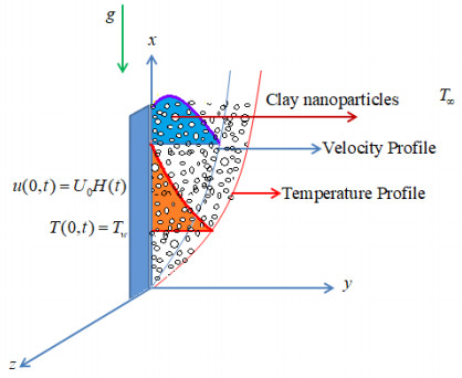
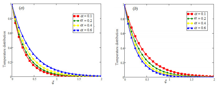
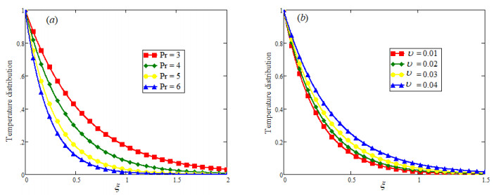
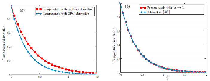
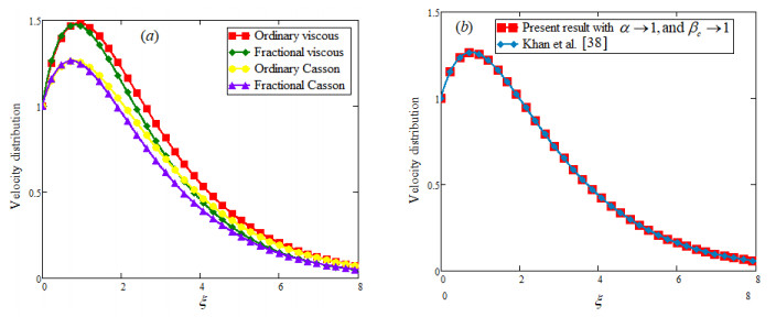
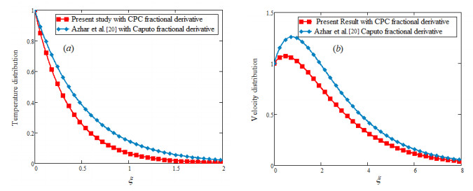
This research article is design to elaborate the rule and significance of fractional derivative for heat transport in drilling of nanofluid. The respective nanofluid formed by the suspension of clay nanoparticles in the base fluids namely Casson fluid. The physical flow phenomenon is demonstrated with the help of partial differential equations by utilizing the respective thermophysical properties of nanoparticles. Also the geometric and thermal conditions are imposed in flow domain. In the governing equations, the partial derivative with respect to time replaced by new hybrid fractional derivative and then solved analytically for temperature and velocity field with the help of Laplace transformed. The obtained solutions for temperature and velocity are presented geometrically by Mathcad software to see the effectiveness of potent parameters. The temperature and velocity present a significant increasing trend for increasing volume fraction parameter. The obtained results for temperature as well as velocity are also compared with the existing literature and it is concluded that field variables with new hybrid fractional derivative, show more decaying trend as compare to the results with Caputo and Caputo-Fabrizio fractional derivatives.
- Casson fluid,
- Clay nanoparticles,
- new,
- vertical plate,
- heat transfer,
- hybrid fractional derivative
Citation: Mushtaq Ahmad, Muhammad Imran Asjad, Ali Akgül, Dumitru Baleanu. Analytical solutions for free convection flow of Casson nanofluid over an infinite vertical plate[J]. AIMS Mathematics, 2021, 6(3): 2344-2358. doi: 10.3934/math.2021142

Related Papers:

Abstract

This research article is design to elaborate the rule and significance of fractional derivative for heat transport in drilling of nanofluid. The respective nanofluid formed by the suspension of clay nanoparticles in the base fluids namely Casson fluid. The physical flow phenomenon is demonstrated with the help of partial differential equations by utilizing the respective thermophysical properties of nanoparticles. Also the geometric and thermal conditions are imposed in flow domain. In the governing equations, the partial derivative with respect to time replaced by new hybrid fractional derivative and then solved analytically for temperature and velocity field with the help of Laplace transformed. The obtained solutions for temperature and velocity are presented geometrically by Mathcad software to see the effectiveness of potent parameters. The temperature and velocity present a significant increasing trend for increasing volume fraction parameter. The obtained results for temperature as well as velocity are also compared with the existing literature and it is concluded that field variables with new hybrid fractional derivative, show more decaying trend as compare to the results with Caputo and Caputo-Fabrizio fractional derivatives.

References

[1]	H. T. Alkasasbeh, M. Z. Swalmeh, A. Hussanan, M. Mamat, Effects of mixed convection on methanol and kerosene oil based micropolar nanofluid containing oxide nanoparticles, CFD Letters, 11 (2019), 55–68.
[2]	A. Raju, O. Ojjela, P. K. Kambhatla, A comparative study of heat transfer analysis on ethylene glycol or engine oil as base fluid with gold nanoparticle in presence of thermal radiation, J. Therm. Anal. Calorim., 2020.
[3]	H. W. Xian, N. Azwadi, C. Sidik, S. R. Aid, T. Ken, Y. Asako, Review on preparation techniques, properties and performance of hybrid nanofluid in recent engineering applications, Journal of Advanced Research in Fluid Mechanics and Thermal Sciences, 45 (2018), 1–13.
[4]	S. Aman, I. Khan, Z. Ismail, M. Z. Salleh, Applications of fractional derivatives to nanofluids: Exact and numerical solutions, Math. Model. Nat. Pheno., 13 (2018), 1–12. doi: 10.1051/mmnp/2018007
[5]	A. Hussanan, N. T. Trung, Heat transfer analysis of sodium Carboxymethyl Cellulose based nanofluid with Tiatania nanoparticles, Journal of Advanced Research in Fluid Mechanics and Thermal Sciences, 56 (2019), 248–256.
[6]	A. Bhattad, J. Sarkar, P. Ghosh, Discrete phase numerical model and experimental study of hybrid nanofluid heat transfer and pressure drop in plate heat exchanger, Int. Commun. Heat Mass, 91 (2018), 262–273. doi: 10.1016/j.icheatmasstransfer.2017.12.020
[7]	K. Farhana, K. Kadirgama, M. M. Noor, M. M. Rahman, D. Ramasamy, A. S. F. Mahamude, CFD modelling of different properties of nanofluids in header and riser tube of flat plate solar collector, In: IOP Conference Series: Materials Science and Engineering, 469 (2019), 012041.
[8]	I. Khan, Shape, effects of MoS2 nanoparticles on MHD slip flow of molybdenum disulphide nanofluid in a porous medium, J. Mol. Liq., 233 (2017), 442–451.
[9]	Z. Shah, P. Kumam, W. Deebani, Radiative MHD Casson Nanofluid flow with Activation energy and chemical reaction over past nonlinearly stretching surface through Entropy generation, Sci. Rep., 10 (2020), 4402. doi: 10.1038/s41598-020-61125-9
[10]	M. Saqib, Convection in ethylene glycol-based molybdenum disulfide nanofluid, J. Therm. Anal. Calorim., 135 (2019), 523–532. doi: 10.1007/s10973-018-7054-9
[11]	J. A. R. Babu, K. K. Kumar, S. S. Rao, State-of-art review on hybrid nanofluids, Renewable and Sustainable Energy Reviews, 77 (2017), 551–565. doi: 10.1016/j.rser.2017.04.040
[12]	N. S. Khan, S. Zuhra, Q. Shah, Entropy generation in two phase model for simulating flow and heat transfer of carbon nanotubes between rotating stretchable disks with cubic autocatalysis chemical reaction, Appl. Nanosci., 9 (2019), 1797–1822. doi: 10.1007/s13204-019-01017-1
[13]	A. Bhattad, J. Sarkar, P. Ghosh, Discrete phase numerical model and experimental study of hybrid nanofluid heat transfer and pressure drop in plate heat exchanger, Int. Commun. Heat Mass, 91 (2018), 262–273. doi: 10.1016/j.icheatmasstransfer.2017.12.020
[14]	S. M. Aminossadati, B. Ghasemi, Natural convection cooling of a localised heat source at the bottom of a nanofluid filled enclosure, Eur. J. Mech. B Fluids, 28 (2009), 630–640. doi: 10.1016/j.euromechflu.2009.05.006
[15]	A. Dawar, Z. Shah, W. Khan, M. Idrees, S. Islam, Unsteady squeezing flow of MHD CNTS nanofluid in rotating channels with Entropy generation and viscous Dissipation, Adv. Mech. Eng., 10 (2019), 1–18.
[16]	M. A. Imran, M. Aleem, M. B. Riaz, R. Ali, I. Khan, A comprehensive report on convective flow of fractional (ABC) and (CF) MHD viscous fluid subject to generalized boundary conditions, Chaos Soliton. Fract., 118 (2019), 274–289. doi: 10.1016/j.chaos.2018.11.016
[17]	J. Hristov, Steady-state heat conduction in a medium with spatial non-singular fading memory, Derivation of Caputo-Fabrizio spacefractional derivative with Jeffreys kernel and analytical solutions, Therm. Sci., 21 (2017), 827–839. doi: 10.2298/TSCI160229115H
[18]	S. Aman, I. Khan, Z. Ismail, M. Z. Salleh, Applications of fractional derivatives to nanofluids: exact and numerical solutions, Math. Model. Nat. Pheno., 13 (2018), 1–12. doi: 10.1051/mmnp/2018007
[19]	N. A. Sheikh, F. Ali, M. Saqib, I. Khan, S. A. Jan, A comparative study of Atangana-Baleanu and Caputo-Fabrizio fractional derivatives to the convective flow of a generalized Casson fluid, Phys. Fluids, 132 (2017), 54–62.
[20]	W. A. Azhar, D. Vieru, C. Fetecau, Free convection flow of some fractional nanofluids over a moving vertical plate with uniform heat flux and heat source, Phys. Fluids, 29 (2017), 082001. doi: 10.1063/1.4996034
[21]	K. A. Abro, M. N. Mirbhar, J. F. Gomez-Aguilar, Functional application of Fourier sine transform in radiating gas flow with non singular and non local kernel, J. Braz. Soc. Mech. Sci. Eng., 41 (2019), 400.
[22]	M. Arif, F. Ali, N. A. Sheikh, I. Khan, K. S. Nisar, Fractional model of couple stress fluid for generalized couette flow: A comparative analysis of Atangana-Baleanu and Caputo-Fabrizio fractional derivatives, IEEE Access, 7 (2019), 88643–88655. doi: 10.1109/ACCESS.2019.2925699
[23]	M. Nazar, M. Ahmad, M. A. Imran, N. A. Shah, Double convection of heat and mass transfer flow of mhd generalized second grade fluid over an exponentially accelerated infinite vertical plate with heat absorption, J. Math. Anal., 8 (2017), 1–10.
[24]	M. Ahmad, M. A. Imran, M. Aleem, I. Khan, A comparative study and analysis of natural convection flow of MHD nonNewtonian fluid in the presence of heat source and first order chemical reaction, J. Therm. Anal. Clorim., 137 (2019), 1783–1796. doi: 10.1007/s10973-019-08065-3
[25]	C. H. Yu, Fractional derivatives of some fractional functions and their applications, Asian Journal of Applied Science and Technology, 4 (2020), 147–158. doi: 10.38177/AJAST.2020.4116
[26]	I. Podlubny, Geometric and physical interpretation of fractional integration and fractional differentiation, Fract. Calc. Appl. Anal., 5 (2002), 367–386.
[27]	N. A. Shah, X. Wang, H. Qi, S. Wang, A. Hajizadeh, Transient electro-osmatic slip flow of an Oldroyd-B fluid with time fractional Caputo-Fabrizio derivative, J. Appl. Comput. Mech., 5 (2019), 779–790.
[28]	C. H. Yu, Fractional derivatives of some fractional functions and their applications, Asian Journal of Applied Science and Technology, 4 (2020), 147–158. doi: 10.38177/AJAST.2020.4116
[29]	D. Baleanu1, J. Alzabut, J. M. Jonnalagadda, Y. Adjabi, M. M. Matar, A coupled system of generalized Sturm-Liouville problems and Langevin fractional differential equations in the framework of nonlocal and nonsingular derivatives, Adv. Differ. Equ., 239 (2020), 1–30.
[30]	D. Baleanu, K. Ghafarnezhad, S. Rezapour, On a strong-singular fractional differential equation, Adv. Differ. Equ., 350 (2020), 1–18.
[31]	A. Atangana, D. Baleanu, New fractional derivatives with non-local and non-singular kernel theory and application to heat transfer model, Therm. Sci., 20 (2016), 763–769. doi: 10.2298/TSCI160111018A
[32]	T. Abdeljawad, A. Fernandez, On a new class of fractional difference-sum operators with discrete Mittag-Leffler kernels, Mathematics, 7 (2019), 1–13.
[33]	F. Jarad, E. Uourlu, T. Abdeljawad, D. Baleanu, On a new class of fractional operators, Adv. Differ. Equ., 1 (2017), 247.
[34]	A. Atangana, A. Akgül, K. M. Owolabi, Analysis of fractal fractional differential equations, Alex. Eng. J., 59 (2020), 2477–2490. doi: 10.1016/j.aej.2020.03.022
[35]	E. K. Akgül, A. Akgül, D. Baleanu, Laplace transform method for economic models with constant proportional Caputo derivative, Fractal Fract., 4 (2020), 1–9.
[36]	M. N. Mirbahar, K. A. Abro, A. W. Shaikh, Calorimetric investigation for thermal plate of Casson fluid via fractional derivative, Journal of Nanofluids, 8 (2019), 1668–1675. doi: 10.1166/jon.2019.1720
[37]	K. A. Abro, I. Khan, K. S. Nisar, A. S. Alsagri, Effects of carbon nanotubes on magnetohydrodynamic flow of methanol based nanofluids via atanganabaleanu and caputo-fabrizio fractional derivatives, Therm. Sci., 23 (2019), 883–898. doi: 10.2298/TSCI180116165A
[38]	I. Khan, A. Hussanan, M. Saqib, S. Shafie, Convective heat transfer in drilling nanofluid with Clay nanoparticles: applications in water cleaning process, BioNanoSci., 9 (2019), 453–460. doi: 10.1007/s12668-019-00623-1
[39]	D. Baleanu, A. Fernandez, A. Akgül, On a fractional operator combining proportional and classical differintegrals, Mathematics, 8 (2020), 360–372. doi: 10.3390/math8030360
[40]	A. Atangana, A. Akgül, K. M. Owolabi, Analysis of fractal fractional differential equations, Alex. Eng. J., 59 (2020), 1117–1134. doi: 10.1016/j.aej.2020.01.005
[41]	A. Atangana, A. Akgül, Can transfer function and Bode diagram be obtained from Sumudu transform, Alex. Eng. J., 59 (2020), 1971–1984. doi: 10.1016/j.aej.2019.12.028
[42]	N. H. Sweilam, S. M. AL-Mekhlafi, D. Baleanu, A hybrid fractional optimal control for a novel Coronavirus (2019-nCov) mathematical model, J. Adv. Res., 2020, In press.
[43]	I. Khan, S. Shafie, Exact solutions for unsteady free convection flow of Casson fluid over an oscillating vertical plate with constant wall temperature, Abstr. Appl. Anal., 2015 (2015), 1–8.
[44]	S. M. Aminossadati, B. Ghasemi, Natural convection cooling of a localised heat source at the bottom of a nanofluidfilled enclosure, Eur. J. Mech. B Fluids, 28 (2009), 630–640. doi: 10.1016/j.euromechflu.2009.05.006
[45]	M. H. Matin, I. Pop, Forced convection heat and mass transfer flow of a nanofluid through a porous channel with a first order chemical reaction on the wall, Int. Commun. Heat Mass, 46 (2013), 134–141. doi: 10.1016/j.icheatmasstransfer.2013.05.001
[46]	H. C. Brinkman, The viscosity of concentrated suspensions and solutions, J. Chem. Phys., 20 (1952), 571–571. doi: 10.1063/1.1700493

Reader Comments

Your name:*

Email:*
© 2021 the Author(s), licensee AIMS Press. This is an open access article distributed under the terms of the Creative Commons Attribution License (http://creativecommons.org/licenses/by/4.0)