Dynamic construction of a family of octic curves as geometric loci

Thierry Dana-Picard; Tomás Recio; Thierry Dana-Picard; Tomás Recio

doi:10.3934/math.2023993

AIMS Mathematics

2023, Volume 8, Issue 8: 19461-19476. doi: 10.3934/math.2023993

Previous Article Next Article

Research article Special Issues

Dynamic construction of a family of octic curves as geometric loci

Thierry Dana-Picard ^{1
,
,},
Tomás Recio ²

1.
Department of Mathematics, Jerusalem College of Technology, Havaad Haleumi Street 21, Jerusalem 9116011, Israel
2.
Universidad Antonio de Nebrija, C/Santa Cruz de Marcenado 27, 28015 Madrid, Spain

Received: 29 March 2023 Revised: 17 May 2023 Accepted: 18 May 2023 Published: 09 June 2023
MSC : 14H50, 51M15, 13P10

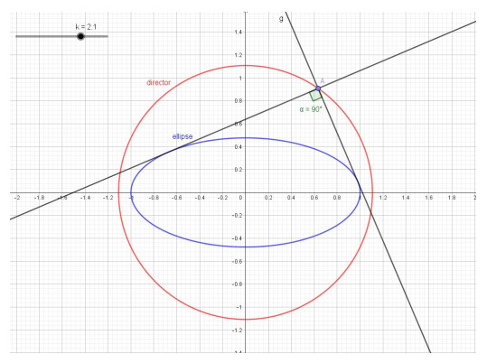
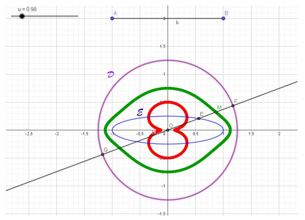
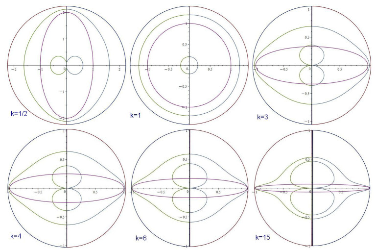
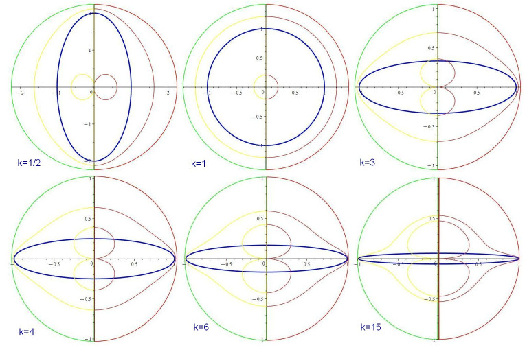
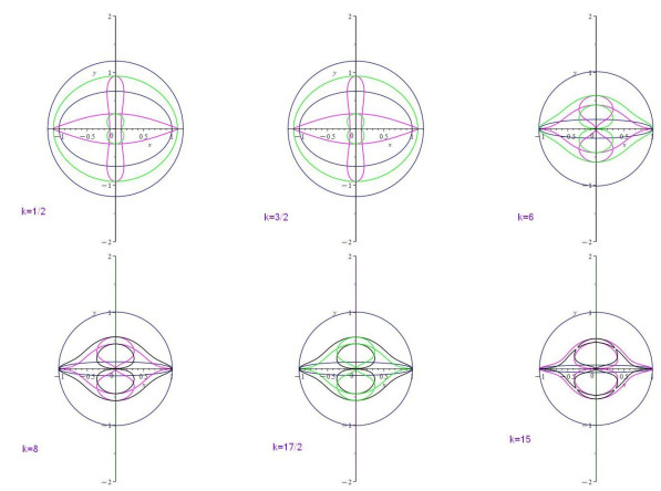
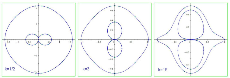
We explore the construction of curves of degree 8 (octics) appearing as geometric loci of points defined by moving points on an ellipse and its director circle. To achieve this goal we develop different computer algebra methods, dealing with trigonometric or with rational parametric representations, as well as through implicit polynomial equations, of the given curves. Finally, we highlight the involved mathematical or computational issues arising when reflecting on the outputs obtained in each case.
- plane curves,
- geometric locus,
- octic curve,
- interactive construction,
- dynamic geometry,
- GeoGebra,
- symbolic computation,
- Maple,
- implicitization
Citation: Thierry Dana-Picard, Tomás Recio. Dynamic construction of a family of octic curves as geometric loci[J]. AIMS Mathematics, 2023, 8(8): 19461-19476. doi: 10.3934/math.2023993

Related Papers:

Abstract

We explore the construction of curves of degree 8 (octics) appearing as geometric loci of points defined by moving points on an ellipse and its director circle. To achieve this goal we develop different computer algebra methods, dealing with trigonometric or with rational parametric representations, as well as through implicit polynomial equations, of the given curves. Finally, we highlight the involved mathematical or computational issues arising when reflecting on the outputs obtained in each case.

References

[1]	M. Abanades, F. Botana, A. Montes, T. Recio, An algebraic taxonomy for locus computation in dynamic geometry, Comput. Aided Design, 56 (2014), 22–33. https://doi.org/10.1016/j.cad.2014.06.008 doi: 10.1016/j.cad.2014.06.008
[2]	J. G. Alcazar, On the shape of rational algebraic curves depending on one parameter, Comput. Aided Geom. D., 27 (2009), 162–178. https://doi.org/10.1016/j.cagd.2009.11.004 doi: 10.1016/j.cagd.2009.11.004
[3]	J. G. Alcazar, J. Schicho, J. R. Sendra, A delineability-based method for Computing Critical Sets of Algebraic Surfaces, J. Symb. Comput., 42 (2007), 678–691. https://doi.org/10.1016/j.jsc.2007.02.001 doi: 10.1016/j.jsc.2007.02.001
[4]	D. Cox, J. Little, D. O'Shea, Ideals, Varieties, and Algorithms: An Introduction to Computational Algebraic Geometry and Commutative Algebra, Undergraduate Texts in Mathematics, NY: Springer, (1992).
[5]	Th. Dana-Picard, Automated study of a regular trifolium, Math. Comput. Sci., 13 (2018), 57–67.
[6]	Th. Dana-Picard, Safety zone in an entertainment park: Envelopes, offsets and a new construction of a Maltese Cross, Electronic Proceedings of the Asian Conference on Technology in Mathematics ACTM 2020; Mathematics and Technology (2020), ISSN 1940–4204 (online version).
[7]	Th. Dana-Picard, Exploration of envelopes of parameterized families of surfaces in a technology-rich environment, Electron. J. Math. Technol., (2023), In press.
[8]	Th. Dana-Picard, S. Hershkovitz, From Space to Maths And to Arts: Virtual Art in Space with Planetary Orbits, Electron. J. Math. Technol., (2023), In press.
[9]	Th. Dana-Picard, Z. Kovács (2021), Networking of technologies: a dialog between CAS and DGS, Electronic J. Math. Technol., 15 (2021), 43–59. https://doi.org/10.1515/econ-2021-0004 doi: 10.1515/econ-2021-0004
[10]	Th. Dana-Picard, Z. Kovács, Dynamic and automated constructions of plane curves, Maple Transactions, (2023), In press.
[11]	Th. Dana-Picard, A. Naiman, W. Mozgawa, V. Ciéslak, Exploring the isoptics of Fermat curves in the affine plane using DGS and CAS, Math. Comput. Sci., 14 (2020), 45–67.
[12]	K. Jin, J. Cheng, On the Complexity of Computing the Topology of Real Algebraic Space Curve, (2023) (preprint). Available from: https://www.researchgate.net/publication/330726079_On_the_Complexity_of_Computing_the_Topology_of_Real_Algebraic_Space_Curves
[13]	Z. Kovács, Th. Dana-Picard, Inner isoptics of a parabola, Conference: 5th Croatian Conference on Geometry and Graphics, Dubrovnik, September 4-8, 2022. Available from: https://www.researchgate.net/publication/363263393_Inner_isoptics_of_a_parabola
[14]	Z. Kovács, B. Parisse, Giac and GeoGebra-improved Gröbner basis computations, In Gutierrez, J., Schicho, J., Weimann, M. (eds.), Computer Algebra and Polynomials, Lecture Notes in Computer Science 8942, (2015), 126–138. Springer. https://doi.org/10.1007/978-3-319-15081-9_7
[15]	E. Roanes-Lozano, E. Roanes-Macías, M. Villar-Mena, A bridge between dynamic geometry and computer algebra, Math. Comput. Model., 37 (2003), 1005–1028. https://doi.org/10.1016/S0895-7177(03)00115-8 doi: 10.1016/S0895-7177(03)00115-8
[16]	E. Roanes-Lozano, N. van Labeke, E. Roanes-Macías, Connecting the 3D DGS Calques3D with the CAS Maple, Math. Comput. Simulat., 80 (2010), 1153–1176. https://doi.org/10.1016/j.matcom.2009.09.008 doi: 10.1016/j.matcom.2009.09.008
[17]	M. Selaković, V. Marinković, P. Janičić, New dynamics in dynamic geometry: Dragging constructed point, J. Symb. Comput., 97 (2020), 3–15.
[18]	J. R. Sendra, F. Winkler, S. Pérez-Díaz, Rational Algebraic Curves: A Computer Algebra Approach, NY: Springer, (2008).
[19]	D. Zeitoun, Th. Dana-Picard, Accurate visualization of graphs of functions of two real variables, Int. J. Comput. Math. Sci., 4 (2010), 1–11.

Reader Comments

Your name:*

Email:*
© 2023 the Author(s), licensee AIMS Press. This is an open access article distributed under the terms of the Creative Commons Attribution License (http://creativecommons.org/licenses/by/4.0)