Research article

Geometry of curve flows in isotropic spaces

  • In this paper, we study inextensible flows of a curve in an isotropic 3-space and give a necessary and sufficient condition for inextensible flows of the curve as a partial differential equation involving the curvatures of the curve. Using binormal flows of a space curve we give the Bäcklund transformations of the Schrödinger flows and the extended Harry-Dym flows. Finally, we investigate some geometric properties of Hasimoto surfaces which wiped out by the Schrödinger flows.

    Citation: Nevin Gürbüz, Dae Won Yoon. Geometry of curve flows in isotropic spaces[J]. AIMS Mathematics, 2020, 5(4): 3434-3445. doi: 10.3934/math.2020222

    Related Papers:

    [1] Ayman Elsharkawy, Clemente Cesarano, Abdelrhman Tawfiq, Abdul Aziz Ismail . The non-linear Schrödinger equation associated with the soliton surfaces in Minkowski 3-space. AIMS Mathematics, 2022, 7(10): 17879-17893. doi: 10.3934/math.2022985
    [2] Zuhal Küçükarslan Yüzbașı, Dae Won Yoon . On geometry of isophote curves in Galilean space. AIMS Mathematics, 2021, 6(1): 66-76. doi: 10.3934/math.2021005
    [3] Nural Yüksel, Burçin Saltık . On inextensible ruled surfaces generated via a curve derived from a curve with constant torsion. AIMS Mathematics, 2023, 8(5): 11312-11324. doi: 10.3934/math.2023573
    [4] Xiaoling Zhang, Cuiling Ma, Lili Zhao . On some $ m $-th root metrics. AIMS Mathematics, 2024, 9(9): 23971-23978. doi: 10.3934/math.20241165
    [5] Hassan Al-Zoubi, Bendehiba Senoussi, Mutaz Al-Sabbagh, Mehmet Ozdemir . The Chen type of Hasimoto surfaces in the Euclidean 3-space. AIMS Mathematics, 2023, 8(7): 16062-16072. doi: 10.3934/math.2023819
    [6] Melek Erdoğdu, Ayșe Yavuz . On differential analysis of spacelike flows on normal congruence of surfaces. AIMS Mathematics, 2022, 7(8): 13664-13680. doi: 10.3934/math.2022753
    [7] Atakan Tuğkan Yakut, Alperen Kızılay . On the curve evolution with a new modified orthogonal Saban frame. AIMS Mathematics, 2024, 9(10): 29573-29586. doi: 10.3934/math.20241432
    [8] Abdelkader Laiadi, Abdelkrim Merzougui . Free surface flows over a successive obstacles with surface tension and gravity effects. AIMS Mathematics, 2019, 4(2): 316-326. doi: 10.3934/math.2019.2.316
    [9] B. B. Chaturvedi, Kunj Bihari Kaushik, Prabhawati Bhagat, Mohammad Nazrul Islam Khan . Characterization of solitons in a pseudo-quasi-conformally flat and pseudo- $ W_8 $ flat Lorentzian Kähler space-time manifolds. AIMS Mathematics, 2024, 9(7): 19515-19528. doi: 10.3934/math.2024951
    [10] Özgür Boyacıoğlu Kalkan, Süleyman Şenyurt, Mustafa Bilici, Davut Canlı . Sweeping surfaces generated by involutes of a spacelike curve with a timelike binormal in Minkowski 3-space. AIMS Mathematics, 2025, 10(1): 988-1007. doi: 10.3934/math.2025047
  • In this paper, we study inextensible flows of a curve in an isotropic 3-space and give a necessary and sufficient condition for inextensible flows of the curve as a partial differential equation involving the curvatures of the curve. Using binormal flows of a space curve we give the Bäcklund transformations of the Schrödinger flows and the extended Harry-Dym flows. Finally, we investigate some geometric properties of Hasimoto surfaces which wiped out by the Schrödinger flows.


    It is well known that many nonlinear phenomena in physics, chemistry and biology are described by dynamics of shapes, such as curves and surfaces, and the time evolution of a curve and a surface has significations in computer vision and image processing. The time evolution of a curve and a surface is described by flows, in particular inextensible flows of a curve and a surface. Physically, inextensible flows give rise to motion which no strain energy is induced. The swinging motion of a cord of fixed length or of a piece of paper carried by the wind, can be described by inextensible flows of a curve and a surface. Also, the flows arise in the context of many problems in computer visions and computer animations [2,7]

    In [5], Hasimoto studied the relation between integrable systems and geometric curve flows and he showed that the non linear Schrödinger equation is equivalent to the binormal notion flow of space curves by using a transformation relating the wave function of the Schrödinger equation to the curvature and torsion of curves (so-called Hasimoto transformation). In particular, Lamb [8] proved that the mKdV equation and the sine-Gordon equation arise from the invariant curve flows by using the Hasimoto transformation. After, Mohamed [9] investigated the general description of the binormal motion of a spacelike and a timelike curve in a 3-dimensional de-Sitter space and gave some explicit examples of a binormal motion of the curves. Schief and Rogers [11] investigated binormal motions of inextensible curves with a constant curvature or a constant torsion, and introduced two new examples of integrable equations which are derived from the binormal motion of curves and established the Bäcklund transformation and matrix Darboux transformations of the extended Dym equation and the mKdV equation. In [1] the authors studied curve motions by the binormal flow with the curvature and the torsion depending velocity and sweeping out immersed surfaces and obtained filaments evolving with a constant torsion which arise from extremal curves of curvature energy functionals. Curve flows have been studied by many experts and geometers [4,6,13].

    The outline of the paper is organized as follows: In Section 2, we give some geometric concepts of curves and surfaces in an isotropic 3-space. In Section 3, we study inextensible flows of a space curve and give time evolutions of the Frenet frame, the curvature and the torsion of the curve. In the last section, we construct the Bäcklund transformations of the Schrödinger flows and the extended Harry-Dym flows as the binormal flows and give a nonexistence of bi-harmonic Hasimoto surfaces in an isotropic 3-space.

    The three dimensional isotropic space I3 has been developed by Strubecker in the 1940s, and it is based on the following group G6 of an affine transformations (x,y,z)(ˉx,ˉy,ˉz) in R3,

    ˉx=a+xcosϕysinϕ,ˉy=b+xsinϕ+ycosϕ,ˉz=c+c1x+c2y+z,

    where a,b,c,c1,c2,ϕR. Such affine transformations are called isotropic congruence transformations or isotropic motions of I3, in this case B6 is denoted by the group of isotropic motions (cf. [12]). Observe that on the xy plane this geometry looks exactly like the plane Euclidean geometry. The projection of a vector x=(x1,y1,z1) in I3 on the xy plane is called the top view of x and we shall denote it by ˆx=(x1,y1,0). The top view concept plays a fundamental role in the isotropic space I3, since the z direction is preserved under action of B6. A line with this direction is called an isotropic line and a plane that contains an isotropic line is said to be an isotropic plane.

    In the sequel, many of metric properties in isotropic geometry (invariants under B6) are Euclidean invariants in the top view such as the isotropic distance, so call i-distance. The isotropic distance of two points P=(x1,y1,z1) and Q=(x2,y2,z2) is defined as the Euclidean distance of the their top views, i.e.,

    d(P,Q):=(x1x2)2+(y1y2)2. (2.1)

    As a fact, two points (x,y,zi) (i=1,2) with the same top views have isotropic distance zero, they called parallel points.

    Let x=(x1,y1,z1) and y=(x2,y2,z2) be vectors in I3. The isotropic inner product of x and y is defined by

    x,y={z1z2,ifxi=0andyi=0x1x2+y1y2,if otherwise. (2.2)

    We call vector of the form x=(0,0,z) in I3 isotropic vector, and non-isotropic vector otherwise.

    Now we introduce some terminology related to curves. A regular curve C:II3, i.e., C0, is parametrized by an arc-length s if ||C||=1. In the following we assume that all curves are parametrized by an arc-length s. In addition, a point α(s0) in which {C(s0),C(s0)} is linearly dependent is an inflection point and a regular unit speed curve C(s)=(x(s),y(s),z(s)) with no inflection point is called an admissible curve if xyxy0.

    On the other hand, the (isotropic) unit tangent, principal normal, and curvature function of the curve C are defined as usual

    t(s)=C(s),n(s)=t(s)κ(s),andκ(s)=||t(s)||=||^t(s)||, (2.3)

    respectively. As usually happens in isotropic geometry, the curvature κ is just the curvature function of its top view ˆC and then we may write κ(s)=(xyxy)(s). To compute the moving trihedron, we define the binormal vector as the vector b=(0,0,1) in the isotropic direction. The Frenet equation corresponding to the isotropic Frenet frame {t,n,b} can be written as ([12])

    dds(tnb)=(0κ0κ0τ000)(tnb), (2.4)

    where τ is the (isotropic) torsion, that is,

    τ=det(C,C,C)κ2.

    Consider a Cr-surface M, r1, in I3 parameterized by

    X(u,v)=(x(u,v),y(u,v),z(u,v)).

    A surface M immersed in I3 is called admissible if it has no isotropic tangent planes. We restrict our framework to admissible regular surfaces.

    For such a surface, the coefficients gij (i,j=1,2) of its first fundamental form are given by

    g11=Xu,Xu,g12=Xu,Xv,g22=Xv,Xv,

    where Xu=Xu and Xv=Xv. The coefficients hij (i,j=1,2) of the second fundamental form of M are calculated with respect to the normal vector of M and they are given by

    h11=det(XuuXuXv)det(gij),h12=det(XuvXuXv)det(gij),h22=det(XvvXuXv)det(gij).

    The isotropic Gaussian curvature K and the isotropic mean curvature H are defined by

    K=det(hij)det(gij),H=g11h222g12h12+g22h112det(gij). (2.5)

    The surface M is said to be isotropic flat (resp. isotropic minimal) if K (resp.H) vanishes (cf. [12,14]).

    We assume that C:[0,l]×[0,w]MI3 is a one parameter family of a space curve in I3, where l is the arc-length of a initial curve. Let u be the curve parametrization variable, 0ul. We put v=||Cu||, from which the arc-length of C is defined by s(u)=u0vdu. Also, the operator s is given in terms of u by s=1vu and the arc-length parameter is given by ds=vdu.

    On the Frenet frame {t,n,b} of the curve C in I3, any flow of C can be given by

    Ct=αt+βn+γb, (3.1)

    where α,β,γ are scalar speeds of the space curve C, respectively. We put s(u,t)=u0vdu, it is called the arc-length variation of C. From this, the requirement that the curve not be subject to any elongation or compression can be expressed by the condition

    ts(u,t)=u0vtdu=0 (3.2)

    for all u[0,l].

    Definition 3.1. A curve evolution C(u,t) and its flow Ct in I3 are said to be inextensible if

    t||Cu||=0.

    Theorem 3.2. If Ct=αt+βn+γb is a flow of C in an isotropic 3-space I3, then we have the following equation:

    vt=αuvκβ. (3.3)

    Proof. Since v2=Cu,Cu and u, t are independent coordinates, u and t commute. So by differentiating of v2 with respect to t and using (2.4) and (3.1) we can easily obtain (3.3).

    Now, we give necessary and sufficient condition for a inextensible flow in an isotropic space and it is useful to get our results.

    Theorem 3.3. Let Ct=αt+βn+γb be a flow of a space curve C in I3. Then the flow is inextensible if and only if

    αs=κβ. (3.4)

    Proof. Suppose that the curve flow of a space curve C is inextensible. From (3.2) and (3.3) we have

    ts(u,t)=u0vtdu=u0(αuvκβ)du=0,forallu[0,l].

    It follows that

    αu=vκβ.

    Since s=1vu, we can obtain (3.4).

    Conversely, by following a similar way as above, the proof is completed.

    Theorem 3.4. Let Ct=αt+βn+γb be a flow of a space curve C in I3. If the flow is inextensible, then a time evolution of the Frenet frame {t,n,b} along a curve C is given by

    ddt(tnb)=(0φ1φ2φ100000)(tnb), (3.5)

    where

    φ1=βs+ακ,φ2=γs+βτ. (3.6)

    Proof. Noting that

    tt=t(Cs)=s(αt+βn+γb)=(βs+ακ)n+(γs+βτ)b. (3.7)

    Also,

    0=tt,n=tt,n+t,nt=(βs+ακ)+t,nt,0=tn,b=nt,b,

    which imply that a time evolution of the principal normal vector n can be expressed as

    nt=(βs+ακ)t.

    This completes the proof.

    Now, we give time evolution equations of the curvature κ and the torsion τ of the inextensible space curve C in I3.

    Theorem 3.5. Let Ct=αt+βn+γb be a flow of a space curve C in I3. Then, the time evolution equations of the functions κ and τ for the inextensible space curve C are given by

    κt=φ1s,τt=κφ2. (3.8)

    Proof. It is well known that the arc length and time derivatives commute. That is,

    s(tt)=s(φ1n+φ2b)=(κφ1)t+(φ1s)n+(φ2s+φ1τ)b,

    and

    t(ts)=t(κn)=(κφ1)t+(κt)n.

    Comparing two equations, we find

    κt=φ1s.

    Also by using s(nt)=t(ns) and following a similar way as above, we can obtain the second equation of (3.8). The proof is completed.

    Remark 3.6. Taking β=κs, by (3.4) one find α=12κ2. From the time evolution of the curvature (3.8) we get

    κt=κsss32κ2κs,

    it follows that the curvature κ evolves according to the mKdV equation

    κt+κsss+32κ2κs=0,

    where κs=κs and κt=κt. The corresponding flow of a curve is

    Ct=12κ2tκsn,

    which is the so-called modified KdV flow [3].

    We give a example of inextensible flow of a curve with constant torsion as follows:

    Example 3.7. Taking τ=τ0 = constant. If we consider

    α=α0,β=β0,γ=β0τ0s+γ0t,

    where α0,β0,γ0 are non zero constants, then the PDE system (3.8) takes the form

    κt=α0κs.

    it follows that one solution of the last equation is

    κ(s,t)=es+α0t.

    Thus, (2.4) and (3.5) imply α0ts=tt and n=e(s+α0t)ts. If we take

    t=(cosh(α0s+t),sinh(α0s+t),α0s+t),

    the vector n is given by

    n(s,t)=α0e(s+α0)(sinh(α0s+t),cosh(α0s+t),1).

    Thus, we can get the family of curves Ct, so we can determine the surface that is generated by this family of curves.

    Qu et al. [10] studied the Bäcklund transformations of geometric curve flows in a Euclidean 3-space R3. In this section, we aim to give the Bäcklund transformations of integrable geometric curve flows by using time evolutions of a curve in an isotropic 3-space I3.

    It is well-known that the Schrödinger flow in a 3-space is given by [5]

    Ct=Cs×Css=κb. (4.1)

    In this case we take (α,β,γ)=(0,0,κ) in (3.1), it follows that (3.5) and (3.8) imply the following theorem:

    Theorem 4.1. The Schrödinger flow (4.1) implies the time evolutions of frame fields, the curvature and the torsion of a space curve C in an isotropic 3-space I3 as follows:

    ddt(tnb)=(00κs000000)(tnb), (4.2)
    ddt(κτ)=(00κs0)(κτ). (4.3)

    We now construct the Bäcklund transformation of the Schrödinger flow (4.1). Considering another curve in I3 related C by

    ˜C(s,t)=C(s,t)+μ(s,t)t+ν(s,t)n+ξ(s,t)b, (4.4)

    where μ,ν and ξ are the smooth functions of s and t. Using (2.4), (4.1) and (4.2), a direct computation leads to

    ˜Cs=(1+μsκν)t+(νs+κμ)n+(ξs+τν)b,˜Ct=μtt+νtn+(κ+ξt+κsμ)b. (4.5)

    Let ˜s be the arclength parameter of the curve ˜C. Then

    d˜s=||~Cs||ds=(1+μsκν)2+(νs+κμ)2ds:=Ωds,

    where Ω is a non zero smooth function. It follows that the unit tangent vector of the curve ˜C is determined by

    ˜t=Φ1t+Φ2n+Φ3b, (4.6)

    where Φ1=Ω1(1+μsκν),Φ2=Ω1(νs+κμ) and Φ3=Ω1(ξs+τν). Differentiating (4.5) with respect to ˜s, we get

    ˜t˜s=Φ1sκΦ2Ωt+Φ2s+κΦ1Ωn+Φ3s+τΦ2Ωb

    which gives the curvature of the curve ˜C:

    ˜κ=||^˜Cs||=(Φ1sκΦ2)2+(Φ2s+κΦ1)2Ω:=ΘΩ. (4.7)

    Thus form (2.3) the Frenet frames of the curve ˜C are given by

    ˜n=Φ1sκΦ2Θt+Φ2s+κΦ1Θn+Φ3s+τΦ2Θb,˜b=(0,0,1). (4.8)

    Assume that the curve ˜C also fulfills the Schrödinger flow, that is,

    ˜Ct=˜κ˜b. (4.9)

    The Bäcklund transformation of the Schrödinger flow with the help of (4.5), (4.8) and (4.9) turns out to be the following result (cf. [10]):

    Theorem 4.2. The Schrödinger flow (4.1) is invariant with respect to the Bäcklund transformation (4.4) in an isotropic 3-space I3 if μ,ν and ξ satisfy the system

    μt=0,νt=0,κ+ξt+κsμ=ΘΩ.

    The extended Harry-Dym flow [11]

    Ct=τ12b (4.10)

    is obtained by setting α=0, β=0 and γ=τ12 in a space curve flow (3.1).

    Theorem 4.3. The extended Harry-Dym flow (4.10) implies the time evolutions of frame fields, the curvature and the torsion of a curve C in an isotropic 3-space I3 as follows:

    ddt(tnb)=(00(τ12)s000000)(tnb), (4.11)
    ddt(κτ)=(00(τ12)s0)(κτ). (4.12)

    We consider the Bäcklund transformation of the extended Harry-Dym flow (4.10)

    ˜C(s,t)=C(s,t)+μ(s,t)t+ν(s,t)n+ξ(s,t)b, (4.13)

    where μ,ν and ξ are the smooth functions of s and t. Differentiating (4.13) with respect to s and t and using (4.11) we get

    ˜Cs=(1+μsκν)t+(νs+κμ)n+(ξs+τν)b,˜Ct=μtt+νtn+(τ12+ξt+μ(τ12)s)b. (4.14)

    Let ˜s be the arclength parameter of the curve ˜C. Then the unit tangent vector of the curve ˜C is given by

    ˜t=Φ1t+Φ2n+Φ3b, (4.15)

    where we put

    Φ1=Ω1(1+μsκν),Φ2=Ω1(νs+κμ),Φ3=Ω1(ξs+τν),Ω=(1+μsκν)2+(νs+κμ)2.

    Differentiating (4.15) with respect to ˜s, we get

    ˜t˜s=Φ1sκΦ2Ωt+Φ2s+κΦ1Ωn+Φ3s+τΦ2Ωb,

    it follows that the curvature of the curve ˜C leads to

    ˜κ=||^˜Cs||=(Φ1sκΦ2)2+(Φ2s+κΦ1)2Ω:=ΘΩ. (4.16)

    Thus form (2.3) the Frenet frames of the curve ˜C are given by

    ˜n=Φ1sκΦ2Θt+Φ2s+κΦ1Θn+Φ3s+τΦ2Θb,˜b=(0,0,1). (4.17)

    Assume that the curve ˜C also fulfills the extended Harry-Dym flow, that is,

    ˜Ct=˜τ12˜b. (4.18)

    The Bäcklund transformation of the extended Harry-Dym flow with the help of (4.14) and (4.17) turns out to be the following result:

    Theorem 4.4. The extended Harry-Dym flow (4.10) is invariant with respect to the Bäcklund transformation (4.13) in an isotropic 3-space I3 if μ,ν and ξ satisfy the system

    μt=0,νt=0,τ12+ξt+μ(τ12)s=ΘΩ.

    Definition 4.5. The surface C(s,t) wiped out by the Schrödinger flow (4.1) is called a Hasimoto surface.

    Sometimes, Eq. (4.1) is called the vortex filament or smoke ring equation, and can be viewed as a dynamical system on the space curves. Since Cs=t and Ct=κb, the first and second fundamental forms of the Hasimoto surface are given by

    I=ds2+κ2dt2,II=κds2.

    In this case κ is non-vanishing everywhere. Thus, we have

    Theorem 4.6. Let C(s,t) be a Hasimoto surface such that C(s,t) is a unit speed curve for all t in an isotropic 3-space I3. Then the surface has zero Gaussian curvature and the mean curvature H=12κ.

    Corollary 4.7. There is no minimal Hasimoto surface in an isotropic 3-space.

    Theorem 4.8. Let C(s,t) be a Hasimoto surface in an isotropic 3-space I3. Then the followings are satisfy:

    (1). s-parameter curves of the surface are non-asymptotic curves.

    (2). s-parameter curves of the surface are geodesic curves.

    Proof. Suppose that C(s,t) is a Hasimoto surface such that C(s,t) is a unit speed curve for all t. It is well known that the normal curvature κn of a s-parameter curve on the surface C(s,t) is given by

    κn=U,Css=n,κn=κ,

    where U=Cs×Ct||Cs×Ct|| is a unit normal vector of the surface. Since κ0, a s-parameter curve is non-asymptotic.

    Also, the geodesic curvature κg of a s-parameter curve on the surface C(s,t) is

    κg=U×Cs,Css=n×t,κn=0,

    it follows that a s-parameter curve is geodesic. The proof is completed.

    Theorem 4.9. Let C(s,t) be a Hasimoto surface in an isotropic 3-space I3. Then the followings are satisfy:

    (1). t-parameter curves of the surface are asymptotic curves.

    (2). t-parameter curves of the surface are geodesic curves.

    Proof. The normal curvature κn and the geodesic curvature κg of a t-parameter curve on the surface C(s,t) are given by

    κn=U,Ctt=n,κtb=0,κg=U×Ct,Ctt=n×κb,κtb=0.

    Thus, a t-parameter curve is asymptotic and geodesic. The proof is completed.

    On the other hand, the mean curvature vector H is given by

    H=HU=12κn, (4.19)

    and Laplacian of the mean curvature vector is expressed as

    ΔH=(2κκs)t+12κ(κ4κ2sκκss)n12(3κsτ+κτs)b. (4.20)

    Theorem 4.10. Let C(s,t) be a Hasimoto surface such that C(s,t) is a unit speed curve for all t in an isotropic 3-space I3. If the surface satisfies the condition ΔH=λH for some constant λ, then the curve C(s,t) for all t has a constant curvature and a constant torsion. Furthermore, λ=κ2.

    Proof. Suppose that a Hasimoto surface satisfies the condition ΔH=λH. With the help of (4.19) and (4.20), we obtain the following equations:

    κκs=0,κ4κ2sκκssλκ2=0,3κsτ+κτs=0, (4.21)

    which imply κs=0 and τs=0. From (4.3) we also get κt=0 and τt=0, that is, κ and τ are constant. Furthermore, from (4.21) λ=κ2. Thus, the proof is completed.

    Corollary 4.11. There is no bi-harmonic Hasimoto surface in an isotropic 3-space.

    Example 4.12. Let us consider the surface in I3 parametrized by

    C(s,t)=(coss,sins,sinscoss+s+t)

    with 0s2π and 2t2. Then, we have

    t(s,t)=(sins,coss,coss+sins+1),n(s,t)=(coss,sins,sins+coss),b(s,t)=(0,0,1),κ(s,t)=1,τ(s,t)=1.

    On the other hand, we can check the following:

    Ct=(0,0,1)=κb,κt=0,τt=0.

    Thus the surface is a Hasimoto surface (Figure 1) and it satisfies ΔH=H.

    Figure 1.  Hasimoto surface with constant curvature and torsion.

    The authors would like to thank the anonymous referee for useful comments and suggestions that helped for a significant improvement of the exposition.

    This paper was supported by Basic Science Research Program through the National Research Foundation of Korea(NRF) funded by the Ministry of Education (NRF-2018R1D1A1B07046979).

    The authors declare no conflicts of interest.


    [1] J. Arroyo, O. J. Garay, A. Pámpano, Binormal motion of curves with constant torsion in 3-spaces, Adv. Math. Phys., 2017 (2017), 1-8. doi: 10.1155/2017/7075831
    [2] M. Desbrun, M. P. Cani-Gascuel, Active implicit surface for animation, In: Proc. Graphics Interface-Canadian Inf. Process. Soc., 1998, 143-150.
    [3] R. E. Goldstein, D. M. Petrich, The Kortewege-de Vries hierachy as dynamics of closed curves in the plane, Phys. Rev. Lett., 67 (1991), 3203-3206. doi: 10.1103/PhysRevLett.67.3203
    [4] N. Gurbuz, Inextensible flows of spacelike, timelike and null curves, Int. J. Contemp. Math. Sci., 4 (2009), 1599-1604.
    [5] H. Hasimoto, A soliton on a vortex filament, J. Fluid Mech., 51 (1972), 477-485. doi: 10.1017/S0022112072002307
    [6] R. A. Hussien, S. G. Mohamed, Generated surfaces via inextensible flows of curves in R3, J. Appl. Math., 2016 (2016), 1-8.
    [7] M. Kass, A. Witkin, D. Terzopoulos, Snakes: Active contour models, In: Proc. 1st Int. Conference on Computer Vision, 1987, 259-268.
    [8] G. L. Lamb Jr, Elements of Soliton Theory, JohnWiley and Sons, New York, 1980.
    [9] S. G. Mohamed, Binormal motions of inextensible curves in de-sitter space S2,1, J. Egyptian Math. Soc., 25 (2017), 313-318.
    [10] C. Qu, J. Han, J. Kang, Bäcklund transformations for integrable geometric curve flows, Symmetry, 7 (2015), 1376-1394. doi: 10.3390/sym7031376
    [11] W. K. Schief, C. Rogers, Binormal motion of curves of constant curvature and torsion. Generation of soliton surfaces, Proc. R. Soc. London Ser. A, 455 (1999), 3163-3188.
    [12] Ž. M. ŠipuŠ, Translation surfaces of constant curvatures in a simpley isotropic space, Period. Math. Hungar., 68 (2014), 160-175. doi: 10.1007/s10998-014-0027-2
    [13] M. Yeneroglu, On new characterization of inextensible flows of space-like curves in de Sitter space, Open Math., 14 (2016), 946-954. doi: 10.1515/math-2016-0071
    [14] D. W. Yoon, J. W. Lee, Linear Weingarten helicoidal surfaces in isotropic space, Symmerty, 8 (2016), 1-7.
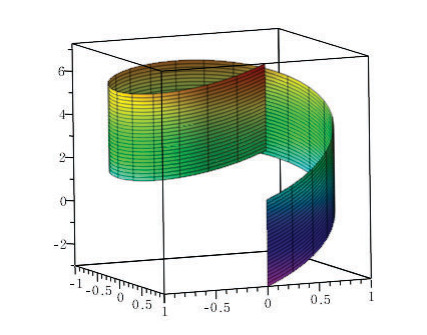
  • This article has been cited by:

    1. Nevin Ertuğ Gürbüz, Ratbay Myrzakulov, Zhaidary Myrzakulova, Three anholonomy densities for three formulations with anholonomic coordinates with hybrid frame in R13, 2022, 261, 00304026, 169161, 10.1016/j.ijleo.2022.169161
    2. Nevin Ertuğ Gürbüz, The evolution of the electric field with Frenet frame in Lorentzian Lie groups, 2021, 247, 00304026, 167989, 10.1016/j.ijleo.2021.167989
    3. Nevin Ertuğ Gürbüz, The evolution of an electric field with respect to the type-1 PAF and the PAFORS frames in R13, 2022, 250, 00304026, 168285, 10.1016/j.ijleo.2021.168285
    4. Nevin Ertuğ Gürbüz, Dae Won Yoon, The visco modified Heisenberg ferromagnet equation and physical applications, 2021, 248, 00304026, 167815, 10.1016/j.ijleo.2021.167815
    5. Nevin Ertug Gürbüz, Zühal Küçükarslan Yüzbası, Dae Won Yoon, Hasimoto Maps for Nonlinear Schrödinger Equations in Minkowski Space, 2022, 29, 1776-0852, 761, 10.1007/s44198-022-00059-4
    6. Nevin Ertuğ Gürbüz, Three geometric phases with the visco-Da Rios equation for the hybrid frame in R13, 2021, 248, 00304026, 168116, 10.1016/j.ijleo.2021.168116
    7. Nevin Ertuğ Gürbüz, Dae Won Yoon, Visco-Da Rios Equation in 3-Dimensional Riemannian Manifold, 2022, 9, 2296-424X, 10.3389/fphy.2021.810920
    8. Nevin Ertuğ Gürbüz, The evolution of an electric field, Hasimoto surfaces and three differential formulas with the new frame in R13, 2023, 272, 00304026, 170217, 10.1016/j.ijleo.2022.170217
    9. Nevin Ertuğ Gürbüz, The null geometric phase along optical fiber for anholonomic coordinates, 2022, 258, 00304026, 168841, 10.1016/j.ijleo.2022.168841
    10. Nevin Ertuğ Gürbüz, The evolution of electric field in pseudo-Galilean 3-space G13, 2022, 269, 00304026, 169818, 10.1016/j.ijleo.2022.169818
    11. W. M. Mahmoud, Esraa. M. Mohamed, M. A. Soliman, Designing and Studying Darboux Sweeping Surface in Isotropic Space I^1_3, 2023, 3, 2732-9976, 1, 10.37394/232021.2023.3.1
    12. Zühal Küçükarslan Yüzbai, Nevin Ertug Gürbüz, Hyun Chul Lee, Dae Won Yoon, Vortex filament flows for curves in a 3-dimensional pseudo-Riemannian manifold, 2024, 0001-9054, 10.1007/s00010-023-01030-4
    13. Ana Savić, Kemal Eren, Soley Ersoy, Vladimir Baltić, Alternative View of Inextensible Flows of Curves and Ruled Surfaces via Alternative Frame, 2024, 12, 2227-7390, 2015, 10.3390/math12132015
  • Reader Comments
  • © 2020 the Author(s), licensee AIMS Press. This is an open access article distributed under the terms of the Creative Commons Attribution License (http://creativecommons.org/licenses/by/4.0)
通讯作者: 陈斌, bchen63@163.com
  • 1. 

    沈阳化工大学材料科学与工程学院 沈阳 110142

  1. 本站搜索
  2. 百度学术搜索
  3. 万方数据库搜索
  4. CNKI搜索

Metrics

Article views(4544) PDF downloads(415) Cited by(13)

Figures and Tables

Figures(1)

Other Articles By Authors

/

DownLoad:  Full-Size Img  PowerPoint
Return
Return

Catalog