Threshold dynamics of a nonlocal diffusion West Nile virus model with spatial heterogeneity

Kangkang Chang; Zhenyu Zhang; Guizhen Liang; Kangkang Chang; Zhenyu Zhang; Guizhen Liang

doi:10.3934/math.2023729

AIMS Mathematics

2023, Volume 8, Issue 6: 14253-14269. doi: 10.3934/math.2023729

Previous Article Next Article

Research article

Threshold dynamics of a nonlocal diffusion West Nile virus model with spatial heterogeneity

1.
School of Mathematics and Statistics, Xinxiang University, Xinxiang 453003, China
2.
Academy of Fine Arts, Xinxiang University, Xinxiang 453003, China

Received: 11 February 2023 Revised: 03 April 2023 Accepted: 06 April 2023 Published: 17 April 2023
MSC : 35B40, 37N25, 92B05

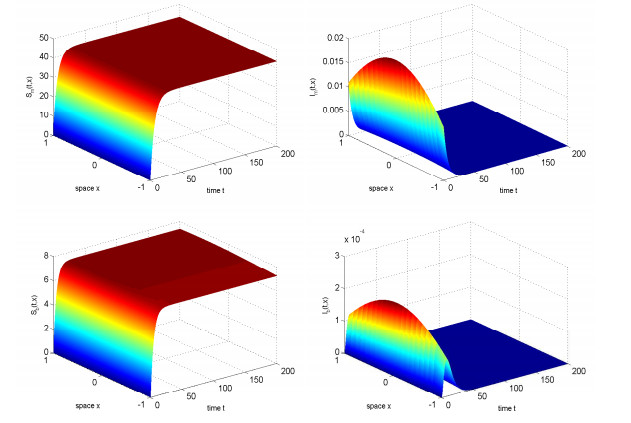
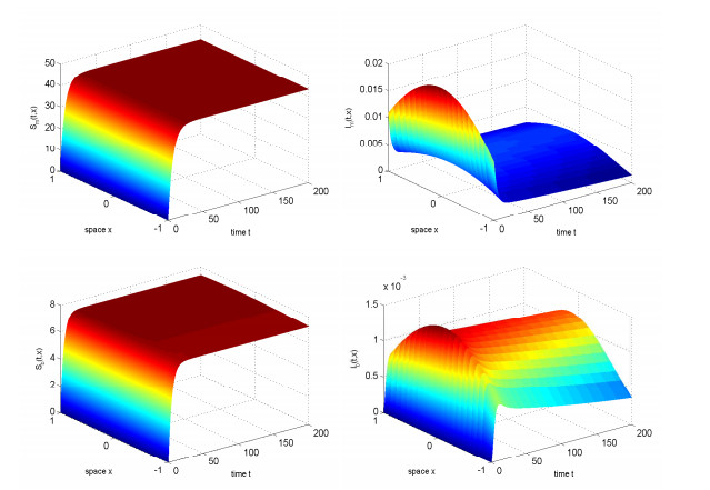
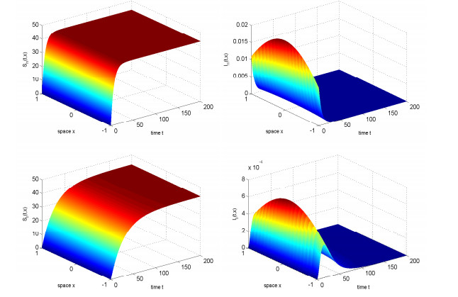
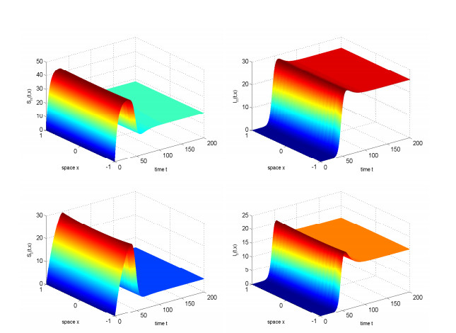
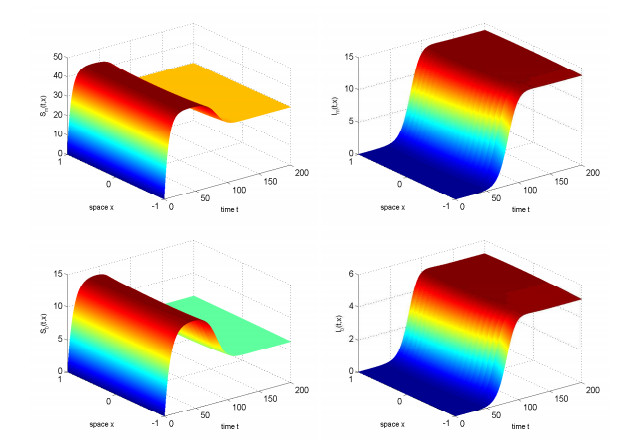
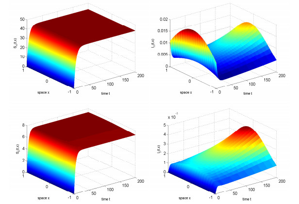
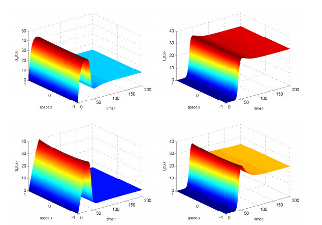
In this study, we investigated the threshold dynamics of a spatially heterogeneous nonlocal diffusion West Nile virus model. By employing semigroup theory and continuous Fréchet-differentiable, we established the well-posedness of the solution. The expression for the basic reproduction number derived using the next-generation matrix method. The authors demonstrated the threshold dynamics of the system by constructing a Lyapunov function and applying the comparison principle. Finally, numerical simulations were used to validate the theorem results. It can be suggested that to control disease development rapidly, measures should be taken to reduce the spread of mosquitoes and birds.
- threshold dynamics,
- nonlocal diffusion,
- West Nile virus model,
- spatial heterogeneity
Citation: Kangkang Chang, Zhenyu Zhang, Guizhen Liang. Threshold dynamics of a nonlocal diffusion West Nile virus model with spatial heterogeneity[J]. AIMS Mathematics, 2023, 8(6): 14253-14269. doi: 10.3934/math.2023729

Related Papers:

Abstract

In this study, we investigated the threshold dynamics of a spatially heterogeneous nonlocal diffusion West Nile virus model. By employing semigroup theory and continuous Fréchet-differentiable, we established the well-posedness of the solution. The expression for the basic reproduction number derived using the next-generation matrix method. The authors demonstrated the threshold dynamics of the system by constructing a Lyapunov function and applying the comparison principle. Finally, numerical simulations were used to validate the theorem results. It can be suggested that to control disease development rapidly, measures should be taken to reduce the spread of mosquitoes and birds.

References

[1]	Chinese Center for Disease Control and Prevention. Available from: https://www.chinacdc.cn/.
[2]	Z. Bai, Z. Zhang, Dynamics of a periodic West Nile virus model with mosquito demographics, Commun. Pure Appl. Anal., 21 (2022), 3755–3775. http://doi.org/10.3934/cpaa.2022121 doi: 10.3934/cpaa.2022121
[3]	J. Ge, Z. Lin, A. K. Tarboush, H. Zhu, Dynamics of West Nile virus driven by seasonal fluctuations in a spatially variable habitat, Discrete Contin. Dyn. Syst. Ser. B, 28 (2023), 2081–2103. http://doi.org/10.3934/dcdsb.2022159 doi: 10.3934/dcdsb.2022159
[4]	S. A. Moon, L. W. Cohnstaedt, D. S. McVey, C. M. Scoglio, A spatio-temporal individual-based network framework for West Nile virus in the USA: spreading pattern of West Nile virus, PLoS Comput. Biol., 15 (2019), e1006875. http://doi.org/10.1371/journal.pcbi.1006875 doi: 10.1371/journal.pcbi.1006875
[5]	A. K. Tarboush, J. Ge, Z. Lin, Coexistence of a cross-diffusive West Nile virus model in a heterogenous environment, Math. Biosci. Eng., 15 (2018), 1479–1494. http://doi.org/10.3934/mbe.2018068 doi: 10.3934/mbe.2018068
[6]	J. Ge, Z. Lin, H. Zhu, Modeling the spread of West Nile virus in a spatially heterogeneous and advective environment, J. Appl. Anal. Comput., 11 (2021), 1868–1897. http://doi.org/10.11948/20200258 doi: 10.11948/20200258
[7]	C. Cheng, Z. Zheng, Spatial and temporal dynamics of an almost periodic reaction-diffusion system for West Nile virus, arXiv: 2012.11789.
[8]	Z. Lin, H. Zhu, Spatial spreading model and dynamics of West Nile virus in birds and mosquitoes with free boundary, J. Math. Biol., 75 (2017), 1381–1409. https://doi.org/10.1007/s00285-017-1124-7 doi: 10.1007/s00285-017-1124-7
[9]	C. Cheng, Z. Zheng, Dynamics and spreading speed of a reaction-diffusion system with advection modeling West Nile virus, J. Math. Anal. Appl., 493 (2021), 124507. https://doi.org/10.1016/j.jmaa.2020.124507 doi: 10.1016/j.jmaa.2020.124507
[10]	M. J. Wonham, T. De-Camino-Beck, M. A. Lewis, An epidemiological model for West Nile virus: invasion analysis and control applications, Proc. R. Soc. Lond. B, 271 (2004), 501–507. https://doi.org/10.1098/rspb.2003.2608 doi: 10.1098/rspb.2003.2608
[11]	A. Abdelrazec, S. Lenhart, H. Zhu, Transmission dynamics of West Nile virus in mosquitoes and corvids and non-corvids, J. Math. Biol., 68 (2014), 1553–1582. https://doi.org/10.1007/s00285-013-0677-3 doi: 10.1007/s00285-013-0677-3
[12]	N. A. Maidana, H. M. Yang, Spatial spreading of West Nile virus described by traveling waves, J. Theor. Biol., 258 (2009), 403–417. https://doi.org/10.1016/j.jtbi.2008.12.032 doi: 10.1016/j.jtbi.2008.12.032
[13]	A. K. Tarboush, Z. Zhang, The diffusive model for West Nile virus on a periodically evolving domain, Complexity, 2020 (2020), 6280313. https://doi.org/10.1155/2020/6280313 doi: 10.1155/2020/6280313
[14]	J. D. Murray, Mathematical biology II: spatial models and biomedical applications, 3 Eds., New York: Springer, 2003. https://doi.org/10.1007/b98869
[15]	J. Garc$\acute{i}$a-Meli$\acute{a}$n, J. D. Rossi, On the principal eigenvalue of some nonlocal diffusion problems, J. Differ. Equations, 246 (2009), 21–38. https://doi.org/10.1016/j.jde.2008.04.015 doi: 10.1016/j.jde.2008.04.015
[16]	Y. Du, W. Ni, Analysis of a West Nile virus model with nonlocal diffusion and free boundaries, Nonlinearity, 33 (2020), 4407–4448. https://doi.org/10.1088/1361-6544/ab8bb2 doi: 10.1088/1361-6544/ab8bb2
[17]	L. Pu, Z. Lin, Y. Lou, A West Nile virus nonlocal model with free boundaries and seasonal succession, J. Math. Biol., 86 (2023), 25. https://doi.org/10.1007/s00285-022-01860-x doi: 10.1007/s00285-022-01860-x
[18]	J. Jiang, Z. Qiu, J. Wu, H. Zhu, Threshold conditions for West Nile virus outbreaks, Bull. Math. Biol., 71 (2009), 627–647. https://doi.org/10.1007/s11538-008-9374-6 doi: 10.1007/s11538-008-9374-6
[19]	A. Pazy, Semigroups of linear operators and applications to partial differential equations, New York: Springer, 1983. https://doi.org/10.1007/978-1-4612-5561-1
[20]	C. Y. Kao, Y. Lou, W. Shen, Random dispersal vs non-local dispersal, Discrete Contin. Dyn. Syst., 26 (2010), 551–596. https://doi.org/10.3934/dcds.2010.26.551 doi: 10.3934/dcds.2010.26.551
[21]	T. Kuniya, J. Wang, Lyapunov functions and global stability for a spatially diffusive SIR epidemic model, Appl. Anal., 96 (2017), 1935–1960. https://doi.org/10.1080/00036811.2016.1199796 doi: 10.1080/00036811.2016.1199796
[22]	G. F. Webb, Theory of nonlinear age-dependent population dynamics, CRC Press, 1985.
[23]	O. Diekmann, J. A. P. Heesterbeek, J. A. Metz, On the definition and the computation of the basic reproduction ratio $R_{0}$ in models for infectious diseases in heterogeneous populations, J. Math. Biol., 28 (1990), 365–382. https://doi.org/10.1007/BF00178324 doi: 10.1007/BF00178324
[24]	V. Hutson, S. Martinez, K. Mischaikow, G. T. Vickers, The evolution of dispersal, J. Math. Biol., 47 (2003), 483–517. https://doi.org/10.1007/s00285-003-0210-1 doi: 10.1007/s00285-003-0210-1
[25]	M. Maliyoni, Probability of disease extinction or outbreak in a stochastic epidemic model for West Nile virus dynamics in birds, Acta Biotheor., 69 (2021), 91–116. https://doi.org/10.1007/s10441-020-09391-y doi: 10.1007/s10441-020-09391-y

Reader Comments

Your name:*

Email:*
© 2023 the Author(s), licensee AIMS Press. This is an open access article distributed under the terms of the Creative Commons Attribution License (http://creativecommons.org/licenses/by/4.0)