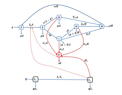
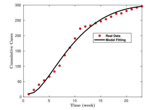
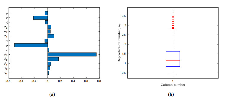
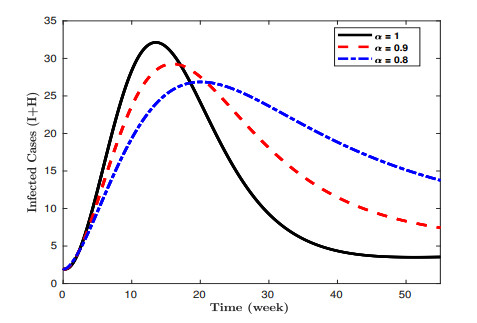
Lassa fever is a fatal zoonotic hemorrhagic disease caused by Lassa virus carried by multimammate rats, which are widely spread in West Africa. In this work, a fractional-order model for Lassa fever transmission dynamics is developed and analysed. The model involves transmissions from rodents-to-human, person-to-person, as well as from Lassa virus infested environment/surfaces. The basic properties of the model such as positivity of solutions, and local stability of the disease-free equilibrium are determined. The reproduction number, $ \mathcal{R}_0 $, of the model is determined using the next generation method and it is used to determine the suitable conditions for disease progression as well as its containment. In addition, we performed sensitivity analysis of the model parameters using the Latin Hypercube Sampling (LHS) scheme to determine the most influential processes on the disease threshold, and determined the key processes to be focused on if the infection is to be curtailed. Moreover, fixed point theory was used to prove the existence and uniqueness of non-trivial solutions of the model. We used the Adams-Bashforth Moulton method to solve the model system numerically for different orders of the fractional derivative. Our results show that using various interventions and control measures such as controlling environmental contamination, reducing rodents-to-humans transmission and interpersonal contact, can significantly help in curbing new infections. Morestill, we observe that an increase in the memory effect, i.e. dependence on future values of the model on the previous states predicts lower peak values of infection cases in the short term, but higher equilibrium values in the long term.
Citation: J. P. Ndenda, J. B. H. Njagarah, S. Shaw. Influence of environmental viral load, interpersonal contact and infected rodents on Lassa fever transmission dynamics: Perspectives from fractional-order dynamic modelling[J]. AIMS Mathematics, 2022, 7(5): 8975-9002. doi: 10.3934/math.2022500
Lassa fever is a fatal zoonotic hemorrhagic disease caused by Lassa virus carried by multimammate rats, which are widely spread in West Africa. In this work, a fractional-order model for Lassa fever transmission dynamics is developed and analysed. The model involves transmissions from rodents-to-human, person-to-person, as well as from Lassa virus infested environment/surfaces. The basic properties of the model such as positivity of solutions, and local stability of the disease-free equilibrium are determined. The reproduction number, $ \mathcal{R}_0 $, of the model is determined using the next generation method and it is used to determine the suitable conditions for disease progression as well as its containment. In addition, we performed sensitivity analysis of the model parameters using the Latin Hypercube Sampling (LHS) scheme to determine the most influential processes on the disease threshold, and determined the key processes to be focused on if the infection is to be curtailed. Moreover, fixed point theory was used to prove the existence and uniqueness of non-trivial solutions of the model. We used the Adams-Bashforth Moulton method to solve the model system numerically for different orders of the fractional derivative. Our results show that using various interventions and control measures such as controlling environmental contamination, reducing rodents-to-humans transmission and interpersonal contact, can significantly help in curbing new infections. Morestill, we observe that an increase in the memory effect, i.e. dependence on future values of the model on the previous states predicts lower peak values of infection cases in the short term, but higher equilibrium values in the long term.

| [1] | Lassa fever. Available from: https://www.ncdc.gov.ng/diseases/factsheet/47. |
| [2] | Lassa fever. Available from: https://www.cdc.gov/vhf/lassa/index.html. |
| [3] | Lassa fever. Available from: https://www.who.int/health-topics/lassa-fever. |
| [4] | K. M. Johnson, T. P. Monath, Imported Lassa fever-reexamining the algorithms, Technical report, Army Medical Research Inst of Infectious diseases Fort Detrick MD, 1990. |
| [5] | M. S. Mahdy, W. Chiang, B. McLaughlin, K. Derksen, B. H. Truxton, K. Neg, Lassa fever: the first confirmed case imported into Canada, Canada diseases weekly report = Rapport hebdomadaire des maladies au Canada, 15 (1989), 193–198. |
| [6] |
R. M. Zweighaft, D. W. Fraser, M. A. W. Hattwick, W. G. Winkler, W. C. Jordan, M. Alter, et al., Lassa fever: response to an imported case, N. Eng. J. Med., 297 (1977), 803–807. http://dx.doi.org/10.1056/NEJM197710132971504 doi: 10.1056/NEJM197710132971504

|
| [7] |
C. M. Hadi, A. Goba, S. H. Khan, J. Bangura, M. Sankoh, S. Koroma, et al., Ribavirin for Lassa fever postexposure prophylaxis, Emerg. Infect. Dis., 16 (2010), 2009–2011. http://dx.doi.org/10.3201/eid1612.100994 doi: 10.3201/eid1612.100994
|
| [8] |
A. R. Akhmetzhanov, Y. Asai, H. Nishiura, Quantifying the seasonal drivers of transmission for Lassa fever in Nigeria, Phil. Trans. R. Soc. B, 374 (2019), 20180268. https://doi.org/10.1098/rstb.2018.0268 doi: 10.1098/rstb.2018.0268
|
| [9] |
I. S. Onah, O. C. Collins, Dynamical system analysis of a Lassa fever model with varying socioeconomic classes, J. Appl. Math., 2020 (2020), 2601706. https://doi.org/10.1155/2020/2601706 doi: 10.1155/2020/2601706
|
| [10] |
J. Mariën, B. Borremans, F. Kourouma, J. Baforday, T. Rieger, S. Günther, et al., Evaluation of rodent control to fight Lassa fever based on field data and mathematical modelling, Emerg. Microbes Infect., 8 (2019), 640–649. https://doi.org/10.1080/22221751.2019.1605846 doi: 10.1080/22221751.2019.1605846
|
| [11] |
E. Fichet-Calvet, D. J. Rogers, Risk maps of Lassa fever in West Africa, PLOS Negl. Trop. Dis., 3 (2009), e388. https://doi.org/10.1371/journal.pntd.0000388 doi: 10.1371/journal.pntd.0000388
|
| [12] | S. Dachollom, C. E. Madubueze, Mathematical model of the transmission dynamics of Lassa fever infection with controls, Math. Model Appl.,, 5 (2020), 65–86. https://doi.org/10.11648/j.mma.20200502.13 |
| [13] |
M. M. Ojo, B. Gbadamosi, T. O. Benson, O. Adebimpe, A. L Georgina, Modeling the dynamics of Lassa fever in Nigeria, J. Egypt Math. Soc., 29 (2021), 1–19. https://doi.org/10.1186/s42787-021-00124-9 doi: 10.1186/s42787-021-00124-9
|
| [14] |
H. Khan, J. F. Gómez-Aguilar, A. Alkhazzan, A. Khan, A fractional order HIV-TB coinfection model with nonsingular Mittag-Leffler Law, Math. Methods Appl. Sci., 43 (2020), 3786–3806. https://doi.org/10.1002/mma.6155 doi: 10.1002/mma.6155
|
| [15] |
S. Patnaik, F. Semperlotti, Application of variable-and distributed-order fractional operators to the dynamic analysis of nonlinear oscillators, Nonlinear Dyn., 100 (2020), 561–580. https://doi.org/10.1007/s11071-020-05488-8 doi: 10.1007/s11071-020-05488-8
|
| [16] |
J. P. Ndenda, J. B. H. Njagarah, S. Shaw, Role of immunotherapy in tumor-immune interaction: Perspectives from fractional-order modelling and sensitivity analysis, Chaos Soliton. Fract., 148 (2021), 111036. https://doi.org/10.1016/j.chaos.2021.111036 doi: 10.1016/j.chaos.2021.111036
|
| [17] |
M. Onal, A. Esen, A Crank-Nicolson approximation for the time fractional Burgers equation, Appl. Math. Nonlinear Sci., 5 (2020), 177–184. https://doi.org/10.2478/amns.2020.2.00023 doi: 10.2478/amns.2020.2.00023
|
| [18] |
J. P. Ndenda, J. B. H. Njagarah, C. B. Tabi, Fractional-Order model for myxomatosis transmission dynamics: Significance of contact, vector control and culling, SIAM J. Appl. Math., 81 (2021), 641–665. https://doi.org/10.1137/20M1359122 doi: 10.1137/20M1359122
|
| [19] |
J. B. H. Njagarah, C. B. Tabi, Spatial synchrony in fractional order metapopulation cholera transmission, Chaos Soliton. Fract., 117 (2018), 37–49. https://doi.org/10.1016/j.chaos.2018.10.004 doi: 10.1016/j.chaos.2018.10.004
|
| [20] |
A. K. Singh, M. Mehra, S. Gulyani, A modified variable-order fractional SIR model to predict the spread of COVID-19 in India, Math. Meth. Appl. Sci., 2021 (2021), 1–15. https://doi.org/10.1002/mma.7655 doi: 10.1002/mma.7655
|
| [21] |
A. Aghili, Complete solution for the time fractional diffusion problem with mixed boundary conditions by operational method, Appl. math. nonlinear sci., 6 (2020), 9–20. https://doi.org/10.2478/amns.2020.2.00002 doi: 10.2478/amns.2020.2.00002
|
| [22] | I. Podlubny, Fractional differential equations: an introduction to fractional derivatives, fractional differential equations, to methods of their solution and some of their applications, Volume 198, $1^ \rm{ st }$ Ed., Elsevier, 1998. |
| [23] | A. A. Kilbas, H. M. Srivastava, J. J. Trujillo, Theory and applications of fractional differential equations, volume 204, $1^\rm{st} $ Ed., Elsevier, 2006. |
| [24] |
D. Kaur, P. Agarwal, M. Rakshit, M. Chand, Fractional calculus involving (p, q)-mathieu type series, Appl. Math. Nonlinear Sci., 5 (2020), 15–34. https://doi.org/10.2478/amns.2020.2.00011 doi: 10.2478/amns.2020.2.00011
|
| [25] |
K. A. Touchent, Z. Hammouch, T. Mekkaoui, A modified invariant subspace method for solving partial differential equations with non-singular kernel fractional derivatives, Appl. Math. Nonlinear Sci., 5 (2020), 35–48. https://doi.org/10.2478/amns.2020.2.00012 doi: 10.2478/amns.2020.2.00012
|
| [26] |
A. O. Akdemir, E. Deniz, E. Yüksel, On some integral inequalities via conformable fractional integrals, Appl. Math. Nonlinear Sci., 6 (2021), 489–498. https://doi.org/10.2478/amns.2020.2.00071 doi: 10.2478/amns.2020.2.00071
|
| [27] |
M. Gürbüz, E. Yldz, Some new inequalities for convex functions via Riemann-Liouville fractional integrals, Appl. Math. Nonlinear Sci., 6 (2021), 537–544. https://doi.org/10.2478/amns.2020.2.00015 doi: 10.2478/amns.2020.2.00015
|
| [28] | H. M. Srivastava, Some parametric and argument variations of the operators of fractional calculus and related special functions and integral transformations, J. Nonlinear Convex Anal,, 22 (2021), 1501–1520. |
| [29] |
H. M. Srivastava, An introductory overview of fractional-calculus operators based upon the Fox-Wright and related higher transcendental functions, J. Adv. Eng. Comput., 5 (2021), 135–166. http://dx.doi.org/10.25073/jaec.202153.340 doi: 10.25073/jaec.202153.340
|
| [30] |
M. Caputo, M. Fabrizio, A new definition of fractional derivative without singular kernel, Progr. Fract. Differ. Appl., 1 (2015), 73–85. https://dx.doi.org/10.12785/pfda/010201 doi: 10.12785/pfda/010201
|
| [31] | A. Atangana, J. F. Gómez-Aguilar, Numerical approximation of Riemann-Liouville definition of fractional derivative: from Riemann-Liouville to Atangana-Baleanu. Numer. Methods Partial Differ. Equ., 34 (2018), 1502–1523. https://doi.org/10.1002/num.22195 |
| [32] |
N. Gul, R. Bilal, E. A. Algehyne, M. G. Alshehri, M. A. Khan, Y. Chu, et al., The dynamics of fractional order Hepatitis B virus model with asymptomatic carriers, Alex. Eng. J., 60 (2021), 3945–3955. https://doi.org/10.1016/j.aej.2021.02.057 doi: 10.1016/j.aej.2021.02.057
|
| [33] |
J. F. Gomez-Aguilar, T. Cordova-Fraga, T. Abdeljawad, A. Khan, H. Khan, Analysis of fractal-fractional malaria transmission model, Fractals, 28 (2020), 2040041. https://doi.org/10.1142/S0218348X20400411 doi: 10.1142/S0218348X20400411
|
| [34] |
E. Uçar, N. Özdemir, A fractional model of cancer-immune system with Caputo and Caputo-Fabrizio derivatives, Eur. Phys. J. Plus, 136 (2021), 1–17. https://doi.org/10.1140/epjp/s13360-020-00966-9 doi: 10.1140/epjp/s13360-020-00966-9
|
| [35] | B. Ghanbari, On the modeling of the interaction between tumor growth and the immune system using some new fractional and fractional-fractal operators, Adv. Differ. Equ., . 2020 (2020), 585. https://doi.org/10.1186/s13662-020-03040-x |
| [36] |
S. T. M. Thabet, M. S. Abdo, K. Shah, Theoretical and numerical analysis for transmission dynamics of COVID-19 mathematical model involving Caputo-Fabrizio derivative, Adv. Differ. Equ., 185 (2021), 1–17. https://doi.org/10.1186/s13662-021-03316-w doi: 10.1186/s13662-021-03316-w
|
| [37] |
S. Rezapour, H. Mohammadi, M. E. Samei, SEIR epidemic model for COVID-19 transmission by Caputo derivative of fractional order, Adv. Differ. Equ., 490 (2020), 1–19. https://doi.org/10.1186/s13662-020-02952-y doi: 10.1186/s13662-020-02952-y
|
| [38] |
D. Baleanu, H. Mohammadi, S. Rezapour, A fractional differential equation model for the COVID-19 transmission by using the Caputo-Fabrizio derivative, Adv Differ Equ., 299 (2020), 1–27. https://doi.org/10.1186/s13662-020-02762-2 doi: 10.1186/s13662-020-02762-2
|
| [39] |
P. A. Naik, M. Yavuz, S. Qureshi, J. Zu, S. Townley, Modeling and analysis of COVID-19 epidemics with treatment in fractional derivatives using real data from Pakistan, Eur. Phys. J. Plus, 135 (2020), 1–42. https://doi.org/10.1140/epjp/s13360-020-00819-5 doi: 10.1140/epjp/s13360-020-00819-5
|
| [40] |
M. ur Rahman, S. Ahmad, R. T. Matoog, N. A. Alshehri, T. Khan, Study on the mathematical modelling of COVID-19 with Caputo-Fabrizio operator, Chaos Soliton. Fract., 150 (2021), 111121. https://doi.org/10.1016/j.chaos.2021.111121 doi: 10.1016/j.chaos.2021.111121
|
| [41] |
T. A. Biala, A. Q. M. Khaliq, A fractional-order compartmental model for the spread of the COVID-19 pandemic, Commun. Nonlinear. Sci. Numer. Simul., 98 (2021), 105764. https://doi.org/10.1016/j.cnsns.2021.105764 doi: 10.1016/j.cnsns.2021.105764
|
| [42] |
H. Singh, H. M. Srivastava, Z. Hammouch, K. S. Nisar, Numerical simulation and stability analysis for the fractional-order dynamics of COVID-19, Results Phys., 20 (2021), 103722. https://doi.org/10.1016/j.rinp.2020.103722 doi: 10.1016/j.rinp.2020.103722
|
| [43] | R. Gorenflo, A. A. Kilbas, F. Mainardi, S. V. Rogosin, Mittag-Leffler functions, related topics and applications, volume 2, Springer, 2014. |
| [44] |
S. Choi, B. Kang, N. Koo, Stability for Caputo fractional differential systems, Abstr. Appl. Anal., 2014 (2014), 631419. https://doi.org/10.1155/2014/631419 doi: 10.1155/2014/631419
|
| [45] |
P. Van den Driessche, J. Watmough, Reproduction numbers and sub-threshold endemic equilibria for compartmental models of disease transmission, Math. Biosci., 180 (2002), 29–48. https://doi.org/10.1016/S0025-5564(02)00108-6 doi: 10.1016/S0025-5564(02)00108-6
|
| [46] |
J. Losada, J. J. Nieto, Properties of a new fractional derivative without singular kernel, Progr. Fract. Differ. Appl., 1 (2015), 87–92. https://dx.doi.org/10.12785/pfda/010202 doi: 10.12785/pfda/010202
|
| [47] |
K. Diethelm, N. J. Ford, A. D. Freed, A predictor-corrector approach for the numerical solution of fractional differential equations, Nonlinear Dynam., 29 (2002), 3–22. https://doi.org/10.1023/A:1016592219341 doi: 10.1023/A:1016592219341
|
| [48] |
K. Diethelm, N. J. Ford, A. D. Freed, Detailed error analysis for a fractional Adams method, Numer. Algorithms, 36 (2004), 31–52. https://doi.org/10.1023/B:NUMA.0000027736.85078.be doi: 10.1023/B:NUMA.0000027736.85078.be
|
| [49] | Population of Nigeria, Available from: https://data.worldbank.org/country/nigeria. |
| [50] |
S. S. Musa, S. Zhao, D. Gao, Q. Lin, G. Chowell, D. He, Mechanistic modelling of the large-scale Lassa fever epidemics in Nigeria from 2016 to 2019, J. Theor. Biol., 493 (2020), 110209. https://doi.org/10.1016/j.jtbi.2020.110209 doi: 10.1016/j.jtbi.2020.110209
|
| [51] |
S. M. Blower, H. Dowlatabadi, Sensitivity and uncertainty analysis of complex models of disease transmission: An HIV model, as an example, Int. Stat. Rev. /Revue Internationale de Statistique, 62 (1994), 229–243. https://doi.org/10.2307/1403510 doi: 10.2307/1403510
|
| [52] |
S. M Kassa, J. B. H Njagarah, Y. A Terefe, Analysis of the mitigation strategies for COVID-19: From mathematical modelling perspective, Chaos Soliton. Fract., 138 (2020), 109968. https://doi.org/10.1016/j.chaos.2020.109968 doi: 10.1016/j.chaos.2020.109968
|
| [53] |
F. Nyabadza, J. B. H. Njagarah, R. J. Smith, Modelling the dynamics of crystal meth ('tik') abuse in the presence of drug-supply chains in South Africa, B. Math. Biol., 75 (2013), 24–48. https://doi.org/10.1007/s11538-012-9790-5 doi: 10.1007/s11538-012-9790-5
|
| [54] |
H. Singh, H. M. Srivastava, Z. Hammouch, K. S. Nisar, Mathematical modeling approach to predict COVID-19 infected people in Sri Lanka, AIMS Math., 7 (2022), 4672–4699. https://doi.org/10.3934/math.2022260 doi: 10.3934/math.2022260
|
Figures(7) / Tables(6)

J. P. Ndenda, J. B. H. Njagarah, S. Shaw. Influence of environmental viral load, interpersonal contact and infected rodents on Lassa fever transmission dynamics: Perspectives from fractional-order dynamic modelling[J]. AIMS Mathematics, 2022, 7(5): 8975-9002. doi: 10.3934/math.2022500


 DownLoad: