Comparison measures for Pythagorean $ m $-polar fuzzy sets and their applications to robotics and movie recommender system

Wiyada Kumam; Khalid Naeem; Muhammad Riaz; Muhammad Jabir Khan; Poom Kumam; Wiyada Kumam; Khalid Naeem; Muhammad Riaz; Muhammad Jabir Khan; Poom Kumam

doi:10.3934/math.2023524

AIMS Mathematics

2023, Volume 8, Issue 5: 10357-10378. doi: 10.3934/math.2023524

Previous Article Next Article

Research article Special Issues

Comparison measures for Pythagorean $ m $-polar fuzzy sets and their applications to robotics and movie recommender system

1.
Applied Mathematics for Science and Engineering Research Unit (AMSERU), Program in Applied Statistics, Department of Mathematics and Computer Science, Faculty of Science and Technology, Rajamangala University of Technology Thanyaburi (RMUTT), Pathum Thani 12110, Thailand
2.
Department of Mathematics, FG Degree College, Lahore Cantt., Pakistan
3.
Department of Mathematics, University of the Punjab, Lahore, Pakistan
4.
Center of Excellence in Theoretical and Computational Science (TaCS-CoE), SCL 802 Fixed Point Laboratory, Science Laboratory Building, King Mongkut's University of Technology Thonburi (KMUTT), 126 Pracha-Uthit Road, Bang Mod, Thung Khru, Bangkok 10140, Thailand
5.
Department of Medical Research, China Medical University Hospital, China Medical University, Taichung 40402, Taiwan

Received: 06 October 2022 Revised: 07 December 2022 Accepted: 10 January 2023 Published: 28 February 2023
MSC : 03E72, 94D05, 90B50

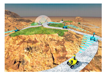
The perception of comparison measures is vitally significant in more or less every scientific field. They have many practical implementations in areas such as medicine, molecular biology, management, meteorology, etc. In this article, novel similarity, distance, and correlation comparison measures for Pythagorean $ m $-polar fuzzy sets are proposed. The leading qualities of these comparison measures are investigated. The numerical examples are provided to demonstrate their formulation. In P$ m $FSs, elements are allowed to duplicate finitely, which supports the usage of the measures put forward in here-and-now situations where we ponder time and again to reach some decision. The three algorithms are proposed to discuss the applications of comparison measures for P$ m $FSs in robotics and movie recommender systems.
- comparison measure,
- Pythagorean $ m $-polar fuzzy sets,
- robotics and movie recommender system
Citation: Wiyada Kumam, Khalid Naeem, Muhammad Riaz, Muhammad Jabir Khan, Poom Kumam. Comparison measures for Pythagorean $ m $-polar fuzzy sets and their applications to robotics and movie recommender system[J]. AIMS Mathematics, 2023, 8(5): 10357-10378. doi: 10.3934/math.2023524

Related Papers:

Abstract

The perception of comparison measures is vitally significant in more or less every scientific field. They have many practical implementations in areas such as medicine, molecular biology, management, meteorology, etc. In this article, novel similarity, distance, and correlation comparison measures for Pythagorean $ m $-polar fuzzy sets are proposed. The leading qualities of these comparison measures are investigated. The numerical examples are provided to demonstrate their formulation. In P$ m $FSs, elements are allowed to duplicate finitely, which supports the usage of the measures put forward in here-and-now situations where we ponder time and again to reach some decision. The three algorithms are proposed to discuss the applications of comparison measures for P$ m $FSs in robotics and movie recommender systems.

References

[1]	L. A. Zadeh, Fuzzy sets, Inform. Control, 8 (1965), 338–353. https://doi.org/10.1016/S0019-9958(65)90241-X doi: 10.1016/S0019-9958(65)90241-X
[2]	L. A. Zadeh, Similarity relations and fuzzy orderings, Inform. Sci., 3 (1971), 177–200. https://doi.org/10.1016/S0020-0255(71)80005-1 doi: 10.1016/S0020-0255(71)80005-1
[3]	L. A. Zadeh, The concept of a linguistic variable and its application to approximate reasoning–I, Inform. Sci., 8 (1975), 199–249. https://doi.org/10.1016/0020-0255(75)90036-5 doi: 10.1016/0020-0255(75)90036-5
[4]	K. T. Atanassov, Intuitionistic fuzzy sets, Fuzzy Sets Syst., 20 (1986), 87–96. https://doi.org/10.1016/S0165-0114(86)80034-3 doi: 10.1016/S0165-0114(86)80034-3
[5]	K. T. Atanassov, More on intuitionistic fuzzy sets, Fuzzy Sets Syst., 33 (1989), 37–45. https://doi.org/10.1016/0165-0114(89)90215-7 doi: 10.1016/0165-0114(89)90215-7
[6]	F. Feng, M. Q. Liang, H. Fujita, R. R. Yager, X. Y. Liu, Lexicographic orders of intuitionistic fuzzy values and their relationships, Mathematics, 7 (2019), 1–26. https://doi.org/10.3390/math7020166 doi: 10.3390/math7020166
[7]	R. R. Yager, Pythagorean fuzzy subsets, In: 2013 Joint IFSA World Congress and NAFIPS Annual Meeting (IFSA/NAFIPS), 2013, 57–61. https://doi.org/10.1109/IFSA-NAFIPS.2013.6608375
[8]	R. R. Yager, A. M. Abbasov, Pythagorean membership grades, complex numbers, and decision making, Int. J. Intell. Syst., 28 (2014), 436–452. https://doi.org/10.1002/int.21584 doi: 10.1002/int.21584
[9]	R. R. Yager, Pythagorean membership grades in multicriteria decision making, IEEE Trans. Fuzzy Syst., 22 (2013), 958–965. https://doi.org/10.1109/TFUZZ.2013.2278989 doi: 10.1109/TFUZZ.2013.2278989
[10]	X. D. Peng, H. Y. Yuan, Y. Yang, Pythagorean fuzzy information measures and their applications, Int. J. Intell. Syst., 32 (2017), 991–1029. https://doi.org/10.1002/int.21880 doi: 10.1002/int.21880
[11]	X. D. Peng, Y. Yang, J. P. Song, Y. Jiang, Pythagorean fuzzy soft set and its application (Chinese), Comput. Eng., 41 (2015), 224–229. https://doi.org/10.3969/j.issn.1000-3428.2015.07.043 doi: 10.3969/j.issn.1000-3428.2015.07.043
[12]	A. Guleria, R. K. Bajaj, On Pythagorean fuzzy soft matrices, operations and their applications in decision making and medical diagnosis, Soft Comput., 23 (2019), 7889–7900. https://doi.org/10.1007/s00500-018-3419-z doi: 10.1007/s00500-018-3419-z
[13]	K. Naeem, M. Riaz, Pythagorean fuzzy soft sets-based MADM, In: Pythagorean fuzzy sets, Singapore: Springer, 2021,407–442. https://doi.org/10.1007/978-981-16-1989-2_16
[14]	K. Naeem, M. Riaz, X. D. Peng, D. Afzal, Pythagorean fuzzy soft MCGDM methods based on TOPSIS, VIKOR and aggregation operators, J. Intell. Fuzzy Syst., 37 (2019), 6937–6957. https://doi.org/10.3233/JIFS-190905 doi: 10.3233/JIFS-190905
[15]	K. Naeem, M. Riaz, D. Afzal, Pythagorean $m$-polar fuzzy sets and TOPSIS method for the selection of advertisement mode, J. Intell. Fuzzy Syst., 37 (2019), 8441–8458. https://doi.org/10.3233/JIFS-191087 doi: 10.3233/JIFS-191087
[16]	K. Naeem, M. Riaz, X. D. Peng, D. Afzal, Pythagorean $m$-polar fuzzy topology with TOPSIS approach in exploring most effectual method for curing from COVID-19, Int. J. Biomath., 13 (2020), 2050075. https://doi.org/10.1142/S1793524520500758 doi: 10.1142/S1793524520500758
[17]	K. Naeem, M. Riaz, F. Karaaslan, Some novel features of Pythagorean $m$-polar fuzzy sets with applications, Complex Intell. Syst., 7 (2021), 459–475. https://doi.org/10.1007/s40747-020-00219-3 doi: 10.1007/s40747-020-00219-3
[18]	M. Riaz, K. Naeem, R. Chinram, A. Iampan, Pythagorean $m$-polar fuzzy weighted aggregation operators and algorithm for the investment strategic decision making, J. Math., 2021 (2021), 6644994. https://doi.org/10.1155/2021/6644994 doi: 10.1155/2021/6644994
[19]	M. Riaz, A. Habib, M. J. Khan, P. Kumam, Correlation coefficients for cubic bipolar fuzzy sets with applications to pattern recognition and clustering analysis, IEEE Access, 9 (2021), 109053–109066. https://doi.org/10.1109/ACCESS.2021.3098504 doi: 10.1109/ACCESS.2021.3098504
[20]	S. Singh, A. H. Ganie, On some correlation coefficients in Pythagorean fuzzy environment with applications, Int. J. Intell. Syst., 35 (2020), 682–717. https://doi.org/10.1002/int.22222 doi: 10.1002/int.22222
[21]	M. J. Khan, M. I. Ali, P. Kumam, W. Kumam, M. Aslam, J. C. R. Alcantud, Improved generalized dissimilarity measure-based VIKOR method for Pythagorean fuzzy sets, Int. J. Intell. Syst., 37 (2022), 1807–1845. https://doi.org/10.1002/int.22757 doi: 10.1002/int.22757
[22]	M. J. Khan, P. Kumam, N. A. Alreshidi, W. Kumam, Improved cosine and cotangent function-based similarity measures for q-rung orthopair fuzzy sets and TOPSIS method, Complex Intell. Syst., 7 (2021), 2679–2696. https://doi.org/10.1007/s40747-021-00425-7 doi: 10.1007/s40747-021-00425-7
[23]	M. Akram, N. Ramzan, A. Luqman, G. Santos-Garcia, An integrated MULTIMOORA method with 2-tuple linguistic Fermatean fuzzy sets: Urban quality of life selection application, AIMS Math., 8 (2023), 2798–2828. https://doi.org/10.3934/math.2023147 doi: 10.3934/math.2023147
[24]	P. Liu, T. Mahmood, Z. Ali, Complex q-rung orthopair fuzzy variation coefficient similarity measures and their approach to medical diagnosis and pattern recognition, Sci. Iran., 29 (2022), 894–914. https://doi.org/10.24200/SCI.2020.55133.4089 doi: 10.24200/SCI.2020.55133.4089
[25]	R. Kausar, H. M. A. Farid, M. Riaz, D. Bozanic, Cancer therapy assessment accounting for heterogeneity using q-rung picture fuzzy dynamic aggregation approach, Symmetry, 14 (2022), 2538. https://doi.org/10.3390/sym14122538 doi: 10.3390/sym14122538
[26]	L. P. Pan, Y. Deng, K. H. Cheong, Quaternion model of Pythagorean fuzzy sets and its distance measure, Expert Syst. Appl., 213 (2023), 119222. https://doi.org/10.1016/j.eswa.2022.119222 doi: 10.1016/j.eswa.2022.119222
[27]	M. Akram, M. Sultan, J. C. R. Alcantud, An integrated ELECTRE method for selection of rehabilitation center with $m$-polar fuzzy N-soft information, Artif. Intell. Med., 135 (2023), 102449. https://doi.org/10.1016/j.artmed.2022.102449 doi: 10.1016/j.artmed.2022.102449
[28]	M. J. Khan, W. Kumam, N. A. Alreshidi, Divergence measures for circular intuitionistic fuzzy sets and their applications, Eng. Appl. Artif. Intell., 116 (2022), 105455. https://doi.org/10.1016/j.engappai.2022.105455 doi: 10.1016/j.engappai.2022.105455
[29]	M. Akram, A. Luqman, J. C. R. Alcantud, An integrated ELECTRE-I approach for risk evaluation with hesitant Pythagorean fuzzy information, Expert Syst. Appl., 200 (2022), 116945. https://doi.org/10.1016/j.eswa.2022.116945 doi: 10.1016/j.eswa.2022.116945
[30]	M. Akram, K. Zahid, J. C. R. Alcantud, A new outranking method for multicriteria decision making with complex Pythagorean fuzzy information, Neural Comput. Appl., 34 (2022), 8069–8102. https://doi.org/10.1007/s00521-021-06847-1 doi: 10.1007/s00521-021-06847-1

Reader Comments

Your name:*

Email:*
© 2023 the Author(s), licensee AIMS Press. This is an open access article distributed under the terms of the Creative Commons Attribution License (http://creativecommons.org/licenses/by/4.0)