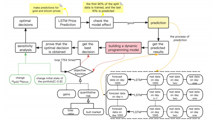
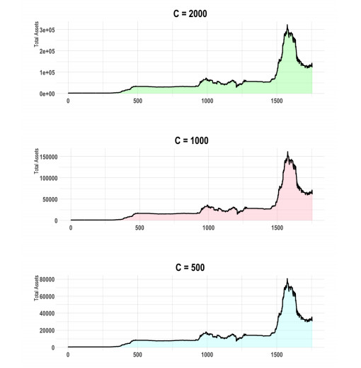
A rational investor always pursues a portfolio with the greatest possible return and the least possible risk. Therefore, a core issue of investment decision analysis is how to make an optimal investment choice in the market with fuzzy information and realize the balance between maximizing the return on assets and minimizing the risk. In order to find optimal investment portfolios of financial assets with high volatility, such as gold and Bitcoin, a mathematical model for formulating investment strategies based on the long short-term memory time series and the dynamic programming model combined with the greedy algorithm has been proposed in this paper. The model provides the optimal daily strategy for the five-year trading period so that it can achieve the maximum expected return every day under the condition of a certain investment amount and a certain risk. In addition, a reasonable risk measure based on historical increases is established while considering the weights brought by different investment preferences. The empirical analysis results show that the optimal total assets and initial capital obtained by the model change in the same proportion, and the model is relatively stable and has strong adaptability to the initial capital. Therefore, the proposed model has practical reference value and research significance for investors and promotes a better combination of computer technology and financial investment decision.
Citation: Jiuchao Ban, Yiran Wang, Bingjie Liu, Hongjun Li. Optimization of venture portfolio based on LSTM and dynamic programming[J]. AIMS Mathematics, 2023, 8(3): 5462-5483. doi: 10.3934/math.2023275
A rational investor always pursues a portfolio with the greatest possible return and the least possible risk. Therefore, a core issue of investment decision analysis is how to make an optimal investment choice in the market with fuzzy information and realize the balance between maximizing the return on assets and minimizing the risk. In order to find optimal investment portfolios of financial assets with high volatility, such as gold and Bitcoin, a mathematical model for formulating investment strategies based on the long short-term memory time series and the dynamic programming model combined with the greedy algorithm has been proposed in this paper. The model provides the optimal daily strategy for the five-year trading period so that it can achieve the maximum expected return every day under the condition of a certain investment amount and a certain risk. In addition, a reasonable risk measure based on historical increases is established while considering the weights brought by different investment preferences. The empirical analysis results show that the optimal total assets and initial capital obtained by the model change in the same proportion, and the model is relatively stable and has strong adaptability to the initial capital. Therefore, the proposed model has practical reference value and research significance for investors and promotes a better combination of computer technology and financial investment decision.

| [1] |
D. G. Baur, T. Dimpfl, K. Kuck, Bitcoin, gold and the us dollar-a replication and extension, Financ. Res. Lett., 25 (2018), 103–110. https://doi.org/10.1016/j.frl.2017.10.012 doi: 10.1016/j.frl.2017.10.012

|
| [2] |
I. Musialkowska, A. Kliber, K. Świerczyńska, P. Marszalek, Looking for a safe-haven in a crisis-driven venezuela: The caracas stock exchange vs gold, oil and bitcoin, Transform. Gov. People, 14 (2020), 475–494. http://doi.org/10.1108/TG-01-2020-0009 doi: 10.1108/TG-01-2020-0009
|
| [3] |
L. Rao, Portfolio selection based on uncertain fractional differential equation, AIMS Mathematics, 7 (2022), 4304–4314. http://doi.org/10.3934/math.2022238 doi: 10.3934/math.2022238
|
| [4] | W. Wang, N. Zhang, D. Fan, X. Wang, Intelligent portfolio optimization based on dynamic trading and risk constraints, J. Cent. Univ. Financ. Econ., 2021, 32–47. |
| [5] |
C. Yang, X. Wang, A steam injection distribution optimization method for sagd oil field using lstm and dynamic programming, ISA T., 110 (2020), 195–248. https://doi.org/10.1016/j.isatra.2020.10.029 doi: 10.1016/j.isatra.2020.10.029
|
| [6] |
N. Zhang, J. Fang, Y. Zhao, Bitcoin price prediction based on lstm hybrid model, Comput. Sci., 48 (2021), 39–45. https://doi.org/10.11896/jsjkx.210600124 doi: 10.11896/jsjkx.210600124
|
| [7] | L. Yang, Y. Wu, J. Wang, Y. Liu, A review of research on recurrent neural networks, Comput. Appl., 38 (2018). |
| [8] |
R. Schnieper, Portfolio optimization, Astin Bull., 30 (2000), 195–248. https://doi.org/10.1007/0-387-24149-3_1 doi: 10.1007/0-387-24149-3_1
|
| [9] |
H. Konno, A. Wijayanayake, Portfolio optimization problem under concave transaction costs and minimal transaction unit constraints, Math. Program., 89 (2001), 233–250. https://doi.org/10.1007/PL00011397 doi: 10.1007/PL00011397
|
| [10] |
Y. Chen, S. Mabu, K. Hirasawa, A model of portfolio optimization using time adapting genetic network programming, Comput. Oper. Res., 37 (2010), 1697–1707. https://doi.org/10.1016/j.cor.2009.12.003 doi: 10.1016/j.cor.2009.12.003
|
| [11] |
G. Ban, N. E. Karoui, A. E. B. Lim, Machine learning and portfolio optimization, Manage. Sci., 64 (2018), 1136–1154. https://doi.org/10.1287/mnsc.2016.2644 doi: 10.1287/mnsc.2016.2644
|
| [12] |
Y. Peng, Y. Liu, R. Zhang, Stock price forecasting modeling and analysis based on lstm, Comput. Eng. Appl., 55 (2019), 209–212. https://doi.org/10.3778/j.issn.1002-8331.1811-0239 doi: 10.3778/j.issn.1002-8331.1811-0239
|
| [13] |
W. Tong, Establishment and solution of linear programming model for venture portfolio, Stat. Decis. Mak., 9 (2016), 89–91. https://doi.org/10.13546/j.cnki.tjyjc.2016.09.022 doi: 10.13546/j.cnki.tjyjc.2016.09.022
|
| [14] |
Y. Fang, Z. Lu, J. Ge, Stock price prediction of joint RMSE loss LSTM-CNN model, Comput. Eng. Appl., 58 (2022), 294-302. https://doi.org/10.3778/j.issn.1002-8331.2112-0006 doi: 10.3778/j.issn.1002-8331.2112-0006
|
Figures(21) / Tables(5)

Jiuchao Ban, Yiran Wang, Bingjie Liu, Hongjun Li. Optimization of venture portfolio based on LSTM and dynamic programming[J]. AIMS Mathematics, 2023, 8(3): 5462-5483. doi: 10.3934/math.2023275


 DownLoad: