The traditional mean-variance portfolio optimization models in practice have suffered from complexity and heavy computation loads in the process of selecting the best assets for constructing a portfolio. If not, they are considerably departed from the theoretically optimized values. In this work, we develop the optimized portfolio investment strategy in which only one asset substitution occurs when re-balancing a portfolio. To do this, we briefly look into a quadratically constrained quadratic programming (QCQP), which has been well-studied for the non-negative solution. Based on the quadratic programming, an efficient scheme is presented for solving the large-scale inverse problem. We more precisely update the rank of an inverse matrix, so that the optimal solution can be easily and quickly obtained by our proposed scheme.
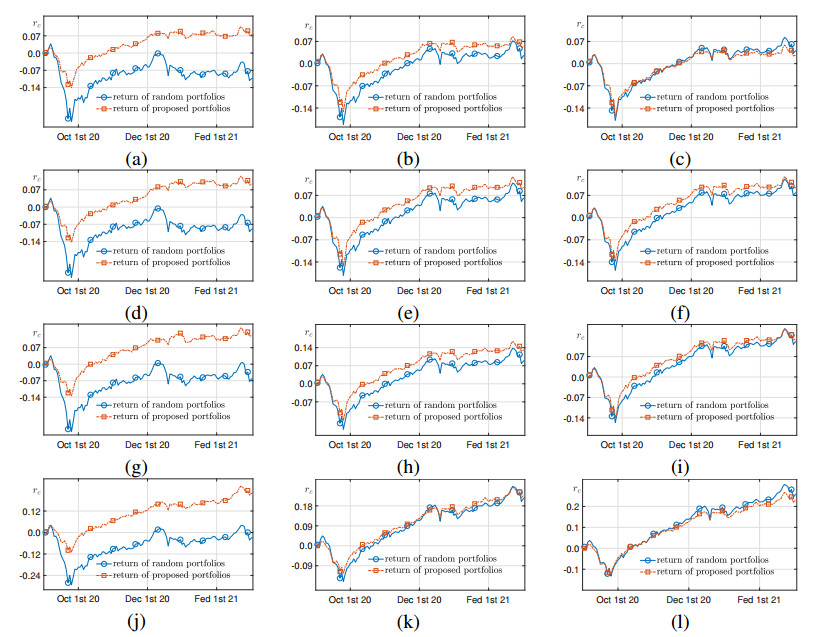
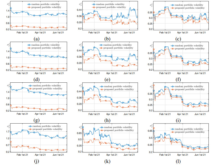
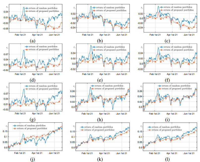
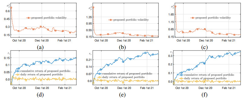
Various numerical and practical experiments are presented to demonstrate the validity and reliability of our scheme. Our empirical application to the U.S. and South Korea stock markets is tested and highlighted. Moreover, comparisons of a random allocation strategy and our proposed scheme reveal the better performance in the lower risks and higher expected returns obtained by our scheme.
Citation: Yunjae Nam, Dongsun Lee. Efficient one asset replacement scheme for an optimized portfolio[J]. AIMS Mathematics, 2022, 7(9): 15881-15903. doi: 10.3934/math.2022869
The traditional mean-variance portfolio optimization models in practice have suffered from complexity and heavy computation loads in the process of selecting the best assets for constructing a portfolio. If not, they are considerably departed from the theoretically optimized values. In this work, we develop the optimized portfolio investment strategy in which only one asset substitution occurs when re-balancing a portfolio. To do this, we briefly look into a quadratically constrained quadratic programming (QCQP), which has been well-studied for the non-negative solution. Based on the quadratic programming, an efficient scheme is presented for solving the large-scale inverse problem. We more precisely update the rank of an inverse matrix, so that the optimal solution can be easily and quickly obtained by our proposed scheme.
Various numerical and practical experiments are presented to demonstrate the validity and reliability of our scheme. Our empirical application to the U.S. and South Korea stock markets is tested and highlighted. Moreover, comparisons of a random allocation strategy and our proposed scheme reveal the better performance in the lower risks and higher expected returns obtained by our scheme.

| [1] |
R. O. Michaud, The Markowitz Optimization Enigma: Is 'Optimized' Optimal? Financ. Anal. J., 45 (1989), 31–42. https://doi.org/10.2469/faj.v45.n1.31 doi: 10.2469/faj.v45.n1.31

|
| [2] |
L. Jiang, S. Wang, Robust multi-period and multi-objective portfolio selection, J. Ind. Manag. Optim., 17 (2021), 695–709. https://doi.org/10.3934/jimo.2019130 doi: 10.3934/jimo.2019130
|
| [3] |
L. Lao, Portfolio selection based on uncertain fractional differential equation, AIMS Math., 7 (2022), 4304–4314. https://doi.org/10.3934/math.2022238 doi: 10.3934/math.2022238
|
| [4] |
H. Huang, Z. Zhang, An intrinsic robust rank-one-approximation approach for currency portfolio optimization, AIMS QFE., 2 (2018), 160–189. https://10.3934/QFE.2018.1.160 doi: 10.3934/QFE.2018.1.160
|
| [5] |
L. Wu, Y. Yang, H. Liu, Non-negative-lasso and application in index tracking, Comput. Stat. Data Anal., 70 (2014), 116–126. https://doi.org/10.1016/j.csda.2013.08.012 doi: 10.1016/j.csda.2013.08.012
|
| [6] |
Y. M. Yen, T. J. Yen, Solving norm constrained portfolio optimization via coordinate-wise descent algorithms, Comput. Stat. Data Anal., 76 (2014), 737–759. https://doi.org/10.1016/j.csda.2013.07.010 doi: 10.1016/j.csda.2013.07.010
|
| [7] |
Z. Dai, J. Kang, F. Wen, Predicting stock returns: a risk measurement perspective, Int. Rev. Financ. Anal., 74 (2021), 101676. https://doi.org/10.1016/j.irfa.2021.101676 doi: 10.1016/j.irfa.2021.101676
|
| [8] |
Z. Dai, J. Kang, Some new efficient mean variance portfolio selection models, International J. Financ. Econ., 74 (2021), 1–13. https://doi.org/10.1002/ijfe.2400 doi: 10.1002/ijfe.2400
|
| [9] |
R. C. Green, B. Hollifield, When will mean-variance efficient portfolios be well diversified?, J. Finance, 47 (1992), 1785–1809. https://doi.org/10.2307/2328996 doi: 10.2307/2328996
|
| [10] |
R. Mansini, W. Ogryczak, M. G. Speranza, Twenty years of linear programming based portfolio optimization, Eur. J. Oper. Res., 234 (2014), 518–535. https://doi.org/10.1016/j.ejor.2013.08.035 doi: 10.1016/j.ejor.2013.08.035
|
| [11] |
C. Aranha, H. Iba, The Memetic Tree-based genetic algorithm and its application to Portfolio Optimization, Menet. Comput., 1 (2009), 139–151. https://doi.org/10.1007/s12293-009-0010-2 doi: 10.1007/s12293-009-0010-2
|
| [12] |
X. Zeng, A stochastic volatility model and optimal portfolio selection, Quant. Financ., 13 (2013), 1547–1558. https://doi.org/10.1080/14697688.2012.740568 doi: 10.1080/14697688.2012.740568
|
| [13] |
A. Buraschi, P. Porchia, F. Trojani, Correlation risk and optimal portfolio choice, J. Financ., 65 (2010), 393–420. http://dx.doi.org/10.2139/ssrn.908664 doi: 10.2139/ssrn.908664
|
| [14] | W. Sun, Y. X. Yuan, Optimization Theory and Methods: Nonlinear Programming, Springer, 2006. |
| [15] |
X. Lin, M. Wang, C. H. Lai, A modification term for Black-Scholes model based on discrepancy calibrated with real market data, AIMS DSFE., 1 (2021), 313–326. https://10.3934/DSFE.2021017 doi: 10.3934/DSFE.2021017
|
| [16] | S. Boyd, Convex optimization, Cambridge University Press, 2004. |
| [17] | R. H. Kwon, Introduction to Linear Optimization and Extensions with MATLAB, CRC Press, 2014. |
| [18] | D. J. Higham, An Introduction to Financial Option Valuation, Cambridge University Press, 2004. |

Figures(10)

Yunjae Nam, Dongsun Lee. Efficient one asset replacement scheme for an optimized portfolio[J]. AIMS Mathematics, 2022, 7(9): 15881-15903. doi: 10.3934/math.2022869


 DownLoad: