The principal-agent model in venture investment based on fairness preference

Dongsheng Xu; Qingqing Liu; Xin Jiang; Dongsheng Xu; Qingqing Liu; Xin Jiang

doi:10.3934/math.2021132

AIMS Mathematics

2021, Volume 6, Issue 3: 2171-2195. doi: 10.3934/math.2021132

Previous Article Next Article

Research article

The principal-agent model in venture investment based on fairness preference

School of Sciences, Southwest Petroleum University, Chengdu, Sichuan 610500, China

Received: 05 August 2020 Accepted: 29 November 2020 Published: 10 December 2020
MSC : 91B08, 91B43

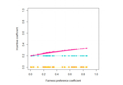
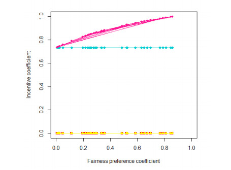
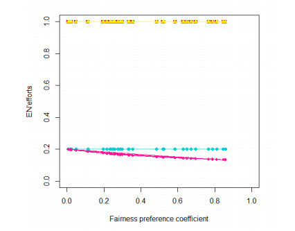
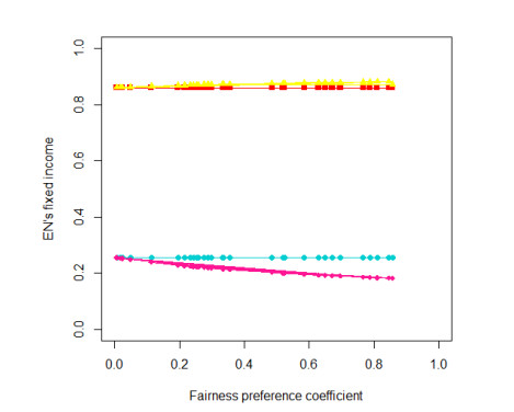
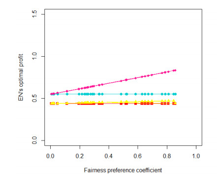
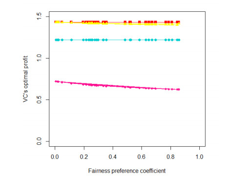
The fairness preference in the principal-agent relationship is a vital factor that can even determine the success or failure of one program. Under normal circumstances, the capital invested by VC is often several times that of EN, which is one of the reasons for the profit gap between EN and VC. Therefore, when establishing a principal-agent model with fairness preferences, it is necessary to project the utility of VC to the level of EN and compare it with the utility of venture entrepreneurs, which will better reflect the profit gap between the two. On the basis of previous studies, this paper considers the amount of contribution of the participants, builds four principal-agent models to find the optimal distribution of income between the Venture Entrepreneur (EN) and the Venture Capital (VC) in a venture capital investment program, two without fairness preference and others with fairness preference. After the simulation we confirm that the fairness preference coefficient exerts a great impact on the distribution of income in both situations where information is symmetric and asymmetric, and a strong fairness preference will lead to a greater net profit gap between the EN and the VC. Thus, the EN should carefully choose the level of his efforts to realize the maximum return for him. In the case of information asymmetry, EN's optimal effort level decreases as the fairness preference coefficient increases.This will affect project revenue. And then affect the VC income.
- Venture Capital,
- principal-agent model,
- fairness preference
Citation: Dongsheng Xu, Qingqing Liu, Xin Jiang. The principal-agent model in venture investment based on fairness preference[J]. AIMS Mathematics, 2021, 6(3): 2171-2195. doi: 10.3934/math.2021132

Related Papers:

Abstract

The fairness preference in the principal-agent relationship is a vital factor that can even determine the success or failure of one program. Under normal circumstances, the capital invested by VC is often several times that of EN, which is one of the reasons for the profit gap between EN and VC. Therefore, when establishing a principal-agent model with fairness preferences, it is necessary to project the utility of VC to the level of EN and compare it with the utility of venture entrepreneurs, which will better reflect the profit gap between the two. On the basis of previous studies, this paper considers the amount of contribution of the participants, builds four principal-agent models to find the optimal distribution of income between the Venture Entrepreneur (EN) and the Venture Capital (VC) in a venture capital investment program, two without fairness preference and others with fairness preference. After the simulation we confirm that the fairness preference coefficient exerts a great impact on the distribution of income in both situations where information is symmetric and asymmetric, and a strong fairness preference will lead to a greater net profit gap between the EN and the VC. Thus, the EN should carefully choose the level of his efforts to realize the maximum return for him. In the case of information asymmetry, EN's optimal effort level decreases as the fairness preference coefficient increases.This will affect project revenue. And then affect the VC income.

References

[1]	G. Moore, Venture capital, Electron. Power, 31 (1985), 558–559.
[2]	P. A. Gompers, Optimal investment, monitoring, and the staging of Venture Capital, J. Finance, 50 (1995), 1461–1489.
[3]	R. Ying, Y. Zhao, An analysis of incentive mechanism and agent cost in venture capital, J. Finance Econ, 30 (2004), 22–29.
[4]	R. Repullo, J. Suarez, Venture Capital Finance: A Security Design Approach, Rev. Financ, 8 (2004), 75–108. doi: 10.1023/B:EUFI.0000022158.96140.f8
[5]	G. Wen-Xin, Double moral hazard and the theory of capital structure of venture capital financing, J. Management Ences. China, 12 (2009), 119–131.
[6]	T. J. Chemmanur, K. Krishnan, D. K. Nandy, How Does Venture Capital Financing Improve Efficiency in Private Firms? A Look Beneath the Surface, Rev. Financ. Stud, 24 (2011), 4037–4090. doi: 10.1093/rfs/hhr096
[7]	S. Kortum, J. Lerner, Assessing the contribution of Venture Capital to innovation, Rand J. Econ, 2000 (31), 674–692.
[8]	S. Srinivasan, I. Barchas, M. Gorenberg, S. Evangelos, Venture Capital: Fueling the innovation economy, Computer, 47 (2014), 40–47.
[9]	Q. shuito, H. bo, A game analysis on the cooperation mechanism between risk investor and risk enterpriser, J. Quant. Techni. Econ, 18 (2001), 60–63.
[10]	C. Casamatta, Financing and advising: Optimal financial contracts with Venture Capitalists, J. Finance, 58 (2003), 2059–2086. doi: 10.1111/1540-6261.00597
[11]	Y. Qing, L. Jue, An analysis of double moral hazard problem and the optimal contract in venture capital financing, Syst. Eng, 22 (2004), 71–73.
[12]	C. Demian, M. Lesheng, W. Bo, The guarding research of risk form principal-agent based on asymmetric information for venture capital, Sci. Management Res, 24 (2006), 106–109.
[13]	D. E. M. Sappington, Incentives in principal-agent relationships, J. Econ. Perspect, 5 (1991), 45–66.
[14]	C. Shujian, X. Jiuping, The study of venture capitals principal-agent model based on asymmetric information, Syst. Eng. Theory Practice, 24 (2004), 20–25.
[15]	W. Liangyong, Z. Huan, Analysis on multi-stage game of the optimal financial contract in Venture Capital investment, Sci. Techno. Management. Res, 32 (2012), 236–239.
[16]	D. Dimov, D. A. Shepherd, K. M. Sutcliffe, Requisite expertise, firm reputation, and status in venture capital investment allocation decisions, J. Bus. Ventur., 22 (2007), 481–502.
[17]	J. Yang, Z. Sun, Y. Liu, Game analysis on the double principal-agent risk in risk investment, IEEE (2009), 159–162.
[18]	H. Wei, A game analysis of adverse selection in venture capital investment, Econ. Management J, (2005), 79–85.
[19]	S. Wang, H. Zhou, Staged financing in venture capital: moral hazard and risks, J. Corporate Finance, 10 (2004), 131–155. doi: 10.1016/S0929-1199(02)00045-7
[20]	Z. Yan, Venture Capitalist-Venture entrepreneur management monitoring model, J. Syst. Management, (2007), 139–143.
[21]	Q. Xiaofeng, Y. Hongying, The Decision Model of Staged Financing in Venture Capital, 2007 International Conference on Wireless Communications, Networking and Mobile Computing, IEEE, (2007), 4153–4156.
[22]	W. Lei, D. Xinghua, W. Xiulai, Research on the influencing factors of control rights allocation in venture capital-backed firms based on the incomplete contract, Sci. Res. Management, 31 (2010), 59–64.
[23]	S. Dahiya, K. Ray, Staged investments in entrepreneurial financing, J. Corporate Finance, 18 (2012), 1193–1216. doi: 10.1016/j.jcorpfin.2012.07.002
[24]	Y. PU, X. GUO, B. CHEN, On incentive mechanism based on fairness preference, Forecasting, 29 (2010), 6–11. doi: 10.1002/for.1146
[25]	E. Fehr, K. M. Schmidt, A Theory of Fairness, Competition and Cooperation, Quarterly J. Econ, 114 (1999), 817–868.
[26]	Z. Yan, C. X. Jian, Principal-agent theory in venture business, Operations Res. Management Sci, (2003), 71–76.
[27]	L. Shanliang, W. Chunhua, Linear Incentive Contract for Principal-agent Problem with Asymmetric Information and Moral Hazard, APCCAS, (2006), 634–637.
[28]	S. D. Zhang, D. X. Wei, Analysis on Multi-stage Investment Game of Double Moral Hazard in Venture Capital, Nankai Econ. Stud, 6 (2008), 142–150.
[29]	W. Liyan, S. Xiaozhong, The Decision Model Research Based on Cooperative Game with Interest Subject of Venture Capital Investment, 2010 First ACIS International Symposium on Cryptography, and Network Security, Data Mining and Knowledge Discovery, E-Commerce and Its Applications, and Embedded Systems. IEEE, (2010), 378–381.
[30]	G. Jun, Y. Yunfeng, Research on the Ways of Improving Principal-Agent Efficiency at Two Levels for Venture Capital, 2009 International Conference on Information Management, Innovation Management and Industrial Engineering. IEEE, (2009), 146–149.
[31]	X. I. Yuqin, Study of Multi-period Dynamic Financial Model of Venture Capital Considering Reputation, Syst. Eng. Theory. Practice, 23 (2003), 76–80.
[32]	W. A. Sahlman, The structure and governance of venture-capital organizations, J. Financ. Econ, 27 (1990), 473–521. doi: 10.1016/0304-405X(90)90065-8
[33]	R. D. Innes, Limited liability and incentive contracting with ex-ante action choices, J. Econ. Theory, 52 (1990), 45–67. doi: 10.1016/0022-0531(90)90066-S
[34]	K. A. Froot, D. S. Scharfstein, J. C. Stein, Risk Management: Coordinating Corporate Investment and Financing Policies, J. Financ, 48 (1993), 1629–1658. doi: 10.1111/j.1540-6261.1993.tb05123.x
[35]	V. A. Dang, Optimal financial contracts with hidden effort, unobservable profits and endogenous costs of effort, Quarterly Rev. Econ. Finance, 50 (2010), 75–89. doi: 10.1016/j.qref.2009.09.005
[36]	E. Lukas, S. Molls, A. Welling, Venture capital, staged financing and optimal funding policies under uncertainty, Eur. J. Oper. Res, 250 (2016), 305–313.
[37]	D. Bergemann, U. Hege, Venture capital financing, moral hazard, and learning, J. Bank Financ., 22 (1998), 6–8.
[38]	J. M. Malcomson, F. Spinnewyn, The multiperiod principal-agent problem, Rev. Econ. Stud, 55 (1988), 391–407. doi: 10.2307/2297391
[39]	C. Xiaohui, W. Wenjuan, D. Ying, To study on decision making on multi-projects and multi-stages portfolio of Venture Capital, Val. Eng, 28 (2009), 106–109.
[40]	Y. Hsu, Staging of Venture Capital investment: A real options analysis, Small Bus. Econ. Group, 35 (2010), 265–281. doi: 10.1007/s11187-008-9158-2
[41]	G. X. Wei, Y. J. Pu, Payment contract design and agency cost analysis based on fairness preference, J. Industrial Eng. Eng. Management, 22 (2008), 58–63.
[42]	J. Zheng, H. Zhong, J. Wu, et al., Research of principle-agent model based on fairness preference in Venture Capital, Int. Conference. Management Serv. Sci, (2010).
[43]	G. Xinyi, An incentive mechanism under fairness preference, 2012 Fifth International Conference on Business Intelligence and Financial Engineering. IEEE, (2012), 438–442.
[44]	J. B. Huang, S. Xu, D. C. Liu, Study on double principal-agent model considering equity incentive based on fairness preference theory, Soft sci, 27 (2013), 124–129.
[45]	D. Chuan, C. Lu, Incentive mechanism for venture investment when venture entrepreneurs have fairness preferences-from explicit efforts and implicit efforts perspectives, J. Management Ences. China, 19 (2016), 104–117.
[46]	W. U. Meng, Venture investment multi stage behavior incentive model of basing on venture entrepreneur having investment fairness concerns, J. Industrial Eng. Eng. Management, 30 (2016), 72–80.
[47]	M. Makris, The theory of incentives: The principal-agent model, Econ. J, 113 (2003).
[48]	L. Heng, Z. Junjun, Study on the incentive model between the venture investor and the venture capitalist based on the principal-agent relationship, J. Quant. Technical Econ, 22 (2005), 151–156.
[49]	S. J. Grossman, O. Hart, An analysis of the principal-agent problem, Econometrica, 51 (1983), 7–45.
[50]	Z. Xubo, Z. Zigang, A Venture Investment Principal-agent Model Base on Game Theory, 2007 IEEE International Conference on Automation and Logistics. IEEE, (2007), 1028–1032.

Reader Comments

Your name:*

Email:*
© 2021 the Author(s), licensee AIMS Press. This is an open access article distributed under the terms of the Creative Commons Attribution License (http://creativecommons.org/licenses/by/4.0)