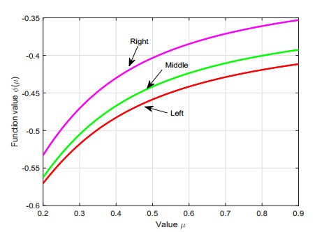
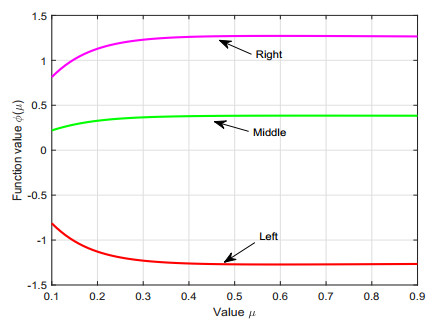
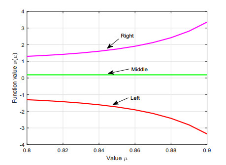
By virtue of the left-sided fractional integral operators having exponential kernels, proposed by Ahmad et al. in [J. Comput. Appl. Math. 353:120-129, 2019], we create the left-sided fractional Hermite–Hadamard type inequalities for convex mappings. Moreover, to study certain fractional trapezoid and midpoint type inequalities via the differentiable convex mappings, two fractional integral identities are proven. Also, we show the important connections of the derived outcomes with those classical integrals clearly. Finally, we provide three numerical examples to verify the correctness of the presented inequalities that occur with the variation of the parameter $ \mu $.
Citation: Shuhong Yu, Tingsong Du. Certain inequalities in frame of the left-sided fractional integral operators having exponential kernels[J]. AIMS Mathematics, 2022, 7(3): 4094-4114. doi: 10.3934/math.2022226
By virtue of the left-sided fractional integral operators having exponential kernels, proposed by Ahmad et al. in [J. Comput. Appl. Math. 353:120-129, 2019], we create the left-sided fractional Hermite–Hadamard type inequalities for convex mappings. Moreover, to study certain fractional trapezoid and midpoint type inequalities via the differentiable convex mappings, two fractional integral identities are proven. Also, we show the important connections of the derived outcomes with those classical integrals clearly. Finally, we provide three numerical examples to verify the correctness of the presented inequalities that occur with the variation of the parameter $ \mu $.

| [1] |
S. Abramovich, L. E. Persson, Fejér and Hermite-Hadamard type inequalities for $N$-quasiconvex functions, Math. Notes, 102 (2017), 599–609. http://dx.doi.org/10.1016/B978-0-12-775850-3.50017-0 doi: 10.1016/B978-0-12-775850-3.50017-0

|
| [2] |
P. Agarwal, Some inequalities involving Hadamard-type $k$-fractional integral operators, Math. Meth. Appl. Sci., 40 (2017), 3882–3891. https://doi.org/10.1002/mma.4270 doi: 10.1002/mma.4270
|
| [3] |
B. Ahmad, A. Alsaedi, M. Kirane, B. T. Torebek, Hermite–Hadamard, Hermite–Hadamard–Fejér, Dragomir–Agarwal and Pachpatte type inequalities for convex functions via new fractional integrals, J. Comput. Appl. Math., 353 (2019), 120–129. https://doi.org/10.1016/j.cam.2018.12.030 doi: 10.1016/j.cam.2018.12.030
|
| [4] |
D. Baleanu, P. O. Mohammed, S. D. Zeng, Inequalities of trapezoidal type involving generalized fractional integrals, Alex. Eng. J., 59 (2020), 2975–2984. https://doi.org/10.1016/j.aej.2020.03.039 doi: 10.1016/j.aej.2020.03.039
|
| [5] |
S. I. Butt, E. Set, S. Yousaf, T. Abdeljawad, W. Shatanawi, Generalized integral inequalities for ABK-fractional integral operators, AIMS Math., 6 (2021), 10164–10191. https://doi.org/10.3934/math.2021589 doi: 10.3934/math.2021589
|
| [6] | H. Chen, U. N. Katugampola, Hermite–Hadamard and Hermite–Hadamard–Fejér type inequalities for generalized fractional integrals, J. Math. Anal. Appl., 446 (2017), 1274–1291. |
| [7] |
F. X. Chen, On the generalization of some Hermite–Hadamard inequalities for functions with convex absolute values of the second derivatives via fractional integrals, Ukrainian Math. J., 70 (2019), 1953–1965. https://doi.org/10.1007/s11253-019-01618-7 doi: 10.1007/s11253-019-01618-7
|
| [8] |
M. R. Delavar, M. D. L. Sen, A mapping associated to $h$-convex version of the Hermite–Hadamard inequality with applications, J. Math. Inequal., 14 (2020), 329–335. https://doi.org/10.2298/PAC2004329S doi: 10.2298/PAC2004329S
|
| [9] | S. S. Dragomir, Two inequalities for differentiable mappings and applications to special means of real numbers and to trapezoidal formula, Appl. Math. Lett., 11 (1998), 91–95. |
| [10] | T. S. Du, M. U. Awan, A. Kashuri, S. S. Zhao, Some $k$-fractional extensions of the trapezium inequalities through generalized relative semi-$(m, h)$-preinvexity, Appl. Anal., 100 (2021), 642–662. |
| [11] | T. S. Du, C. Y. Luo, B. Yu, Certain quantum estimates on the parameterized integral inequalities and their applications, J. Math. Inequal., 15 (2021), 201–228. |
| [12] | T. S. Du, H. Wang, M. A. Khan, Y. Zhang, Certain integral inequalities considering generalized $m$-convexity on fractal sets and their applications, Fractals, 27 (2019), 1–17. |
| [13] |
D. Y. Hwang, S. S. Dragomir, Extensions of the Hermite–Hadamard inequality for $r$-preinvex functions on an invex set, Bull. Aust. Math. Soc., 95 (2017), 412–423. https://doi.org/10.1017/S0004972716001374 doi: 10.1017/S0004972716001374
|
| [14] |
M. Iqbal, M. I. Bhatti, K. Nazeer, Generalization of inequalities analogous to Hermite-Hadamard inequality via fractional integrals, Bull. Korean Math. Soc., 52 (2015), 707–716. https://doi.org/10.4134/BKMS.2015.52.3.707 doi: 10.4134/BKMS.2015.52.3.707
|
| [15] |
İ. İșcan, Weighted Hermite-Hadamard-Mercer type inequalities for convex functions, Numer. Meth. Part. D. E., 37 (2021), 118–130. https://doi.org/10.1002/num.22521 doi: 10.1002/num.22521
|
| [16] |
M. Jleli, D. O'Regan, B. Samet, On Hermite-Hadamard type inequalities via generalized fractional integrals, Turkish J. Math., 40 (2016), 1221–1230. https://doi.org/10.3906/mat-1507-79 doi: 10.3906/mat-1507-79
|
| [17] |
M. Kadakal, İ. İșcan, P. Agarwal, M. Jleli, Exponential trigonometric convex functions and Hermite–Hadamard type inequalities, Math. Slovaca, 71 (2021), 43–56. https://doi.org/10.1515/ms-2017-0410 doi: 10.1515/ms-2017-0410
|
| [18] |
M. A. Khan, T. Ali, S. S. Dragomir, M. Z. Sarikaya, Hermite–Hadamard type inequalities for conformable fractional integrals, Rev. R. Acad. Cienc. Exactas Fís. Nat. Ser. A Math. RACSAM, 112 (2018), 1033–1048. https://doi.org/10.1007/s13398-017-0408-5 doi: 10.1007/s13398-017-0408-5
|
| [19] | M. A. Khan, Y. M. Chu, A. Kashuri, R. Liko, G. Ali, Conformable fractional integrals versions of Hermite–Hadamard inequalities and their generalizations, J. Funct. Spaces, 2018 (2018), Article ID 6928130. |
| [20] |
U. S. Kirmaci, Inequalities for differentiable mappings and applications to special means of real numbers and to midpoint formula, Appl. Math. Comput., 147 (2004), 137–146. https://doi.org/10.1016/S0096-3003(02)00657-4 doi: 10.1016/S0096-3003(02)00657-4
|
| [21] |
M. Kunt, İ. İșcan, S. Turhan, D. Karapinar, Improvement of fractional Hermite–Hadamard type inequality for convex functions, Miskolc Math. Notes, 19 (2018), 1007–1017. https://doi.org/10.18514/MMN.2018.2441 doi: 10.18514/MMN.2018.2441
|
| [22] | M. Kunt, D. Karapinar, S. Turhan, İ. İșcan, The right Riemann–Liouville fractional Hermite–Hadamard type inequalities for convex functions, J. Inequal. Spec. Funct., 9 (2018), 45–57. |
| [23] |
M. Kunt, D. Karapinar, S. Turhan, İ. İșcan, The left Riemann–Liouville fractional Hermite–Hadamard type inequalities for convex functions, Math. Slovaca, 69 (2019), 773–784. https://doi.org/10.1515/ms-2017-0261 doi: 10.1515/ms-2017-0261
|
| [24] |
M. A. Latif, On some new inequalities of Hermite–Hadamard type for functions whose derivatives are $s$-convex in the second sense in the absolute value, Ukrainian Math. J., 67 (2016), 1552–1571. https://doi.org/10.1007/s11253-016-1172-y doi: 10.1007/s11253-016-1172-y
|
| [25] |
J. G. Liao, S. H. Wu, T. S. Du, The Sugeno integral with respect to $\alpha$-preinvex functions, Fuzzy Set. Syst., 379 (2020), 102–114. https://doi.org/10.1016/j.fss.2018.11.008 doi: 10.1016/j.fss.2018.11.008
|
| [26] |
D. Ș. Marinescu, M. Monea, A very short proof of the Hermite–Hadamard inequalities, Amer. Math. Monthly, 127 (2020), 850–851. https://doi.org/10.1080/00029890.2020.1803648 doi: 10.1080/00029890.2020.1803648
|
| [27] |
M. Matłoka, Inequalities for $h$-preinvex functions, Appl. Math. Comput., 234 (2014), 52–57. https://doi.org/10.1016/j.amc.2014.02.030 doi: 10.1016/j.amc.2014.02.030
|
| [28] | K. Mehrez, P. Agarwal, New Hermite-Hadamard type integral inequalities for convex functions and their applications, J. Comput. Appl. Math., 350 (2019), 274–285. |
| [29] | P. O. Mohammed, Hermite–Hadamard inequalities for Riemann–Liouville fractional integrals of a convex function with respect to a monotone function, Math. Meth. Appl. Sci., 44 (2021), 2314–2324. |
| [30] | C. E. M. Pearce, J. Pečarić, Inequalities for differentiable mappings with application to special means and quadrature formulæ, Appl. Math. Lett., 13 (2000), 51–55. |
| [31] | S. Qaisar, J. Nasir, S. I. Butt, A. Asma, F. Ahmad, M. Iqbal, S. Hussain, Some fractional integral inequalities of type Hermite–Hadamard through convexity, J. Inequal. Appl., 2019 (2019), Article Number 111. |
| [32] |
S. Rashid, D. Baleanu, M. C. Yu, Some new extensions for fractional integral operator having exponential in the kernel and their applications in physical systems, Open Physics, 18 (2020), 478–491. https://doi.org/10.1515/phys-2020-0114 doi: 10.1515/phys-2020-0114
|
| [33] |
M. Shafiya, G. Nagamani, D. Dafik, Global synchronization of uncertain fractional-order BAM neural networks with time delay via improved fractional-order integral inequality, Math. Comput. Simulation, 191 (2021), 168–186. https://doi.org/10.1016/j.matcom.2021.08.001 doi: 10.1016/j.matcom.2021.08.001
|
| [34] |
M. Z. Sarikaya, E. Set, H. Yaldiz, N. Bașak, Hermite–Hadamard's inequalities for fractional integrals and related fractional inequalities, Math. Comput. Model., 57 (2013), 2403–2407. https://doi.org/10.1016/j.mcm.2011.12.048 doi: 10.1016/j.mcm.2011.12.048
|
| [35] |
E. Set, A. O. Akdemir, M. E. Özdemir, Simpson type integral inequalities for convex functions via Riemann–Liouville integrals, Filomat, 31 (2017), 4415–4420. https://doi.org/10.2298/FIL1714415S doi: 10.2298/FIL1714415S
|
| [36] | E. Set, J. Choi, B. Çelİk, Certain Hermite-Hadamard type inequalities involving generalized fractional integral operators, Rev. R. Acad. Cienc. Exactas Fís. Nat. Ser. A Mat., 112 (2018), 1539–1547. |
| [37] | W. B. Sun, Q. Liu, New Hermite-Hadamard type inequalities for $(\alpha, m)$-convex functions and applications to special means, J. Math. Inequal., 11 (2017), 383–397. |
| [38] |
J. R. Wang, J. H. Deng, M. Fečkan, Exploring $s$-$e$-condition and applications to some Ostrowski type inequalities via Hadamard fractional integrals, Math. Slovaca, 64 (2014), 1381–1396. https://doi.org/10.2478/s12175-014-0281-z doi: 10.2478/s12175-014-0281-z
|
| [39] |
S. S. Zeid, Approximation methods for solving fractional equations, Chaos, Solitons Fractals, 125 (2019), 171–193. https://doi.org/10.1016/j.chaos.2019.05.008 doi: 10.1016/j.chaos.2019.05.008
|
Figures(3)

Shuhong Yu, Tingsong Du. Certain inequalities in frame of the left-sided fractional integral operators having exponential kernels[J]. AIMS Mathematics, 2022, 7(3): 4094-4114. doi: 10.3934/math.2022226


 DownLoad: