An inertial parallel algorithm for a finite family of $ G $-nonexpansive mappings applied to signal recovery

Nipa Jun-on; Raweerote Suparatulatorn; Mohamed Gamal; Watcharaporn Cholamjiak; Nipa Jun-on; Raweerote Suparatulatorn; Mohamed Gamal; Watcharaporn Cholamjiak

doi:10.3934/math.2022102

AIMS Mathematics

2022, Volume 7, Issue 2: 1775-1790. doi: 10.3934/math.2022102

Previous Article Next Article

Research article

An inertial parallel algorithm for a finite family of $ G $-nonexpansive mappings applied to signal recovery

1.
Faculty of Sciences, Lampang Rajabhat University, Lampang 52100, Thailand
2.
Department of Mathematics, Faculty of Science, Chiang Mai University, Chiang Mai 50200, Thailand
3.
Department of Mathematics, Faculty of Science, South Valley University, Qena 83523, Egypt
4.
School of Science, University of Phayao, Phayao 56000, Thailand

Received: 11 June 2021 Accepted: 04 October 2021 Published: 02 November 2021
MSC : 47H04, 47H10

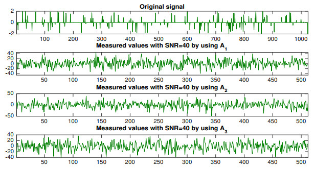
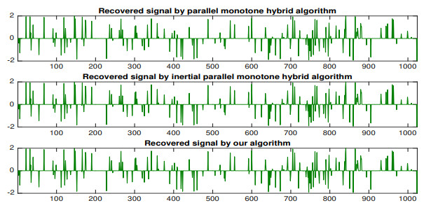
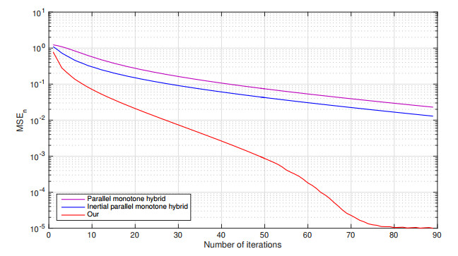
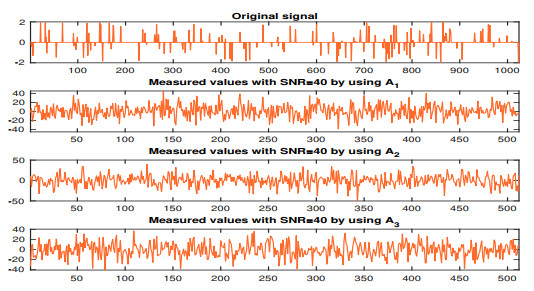
This study investigates the weak convergence of the sequences generated by the inertial technique combining the parallel monotone hybrid method for finding a common fixed point of a finite family of $ G $-nonexpansive mappings under suitable conditions in Hilbert spaces endowed with graphs. Some numerical examples are also presented, providing applications to signal recovery under situations without knowing the type of noises. Besides, numerical experiments of the proposed algorithms, defined by different types of blurred matrices and noises on the algorithm, are able to show the efficiency and the implementation for LASSO problem in signal recovery.
- weak convergence,
- parallel algorithm,
- $ G $-nonexpansive,
- inertial extrapolation,
- numerical discussion
Citation: Nipa Jun-on, Raweerote Suparatulatorn, Mohamed Gamal, Watcharaporn Cholamjiak. An inertial parallel algorithm for a finite family of $ G $-nonexpansive mappings applied to signal recovery[J]. AIMS Mathematics, 2022, 7(2): 1775-1790. doi: 10.3934/math.2022102

Related Papers:

Abstract

This study investigates the weak convergence of the sequences generated by the inertial technique combining the parallel monotone hybrid method for finding a common fixed point of a finite family of $ G $-nonexpansive mappings under suitable conditions in Hilbert spaces endowed with graphs. Some numerical examples are also presented, providing applications to signal recovery under situations without knowing the type of noises. Besides, numerical experiments of the proposed algorithms, defined by different types of blurred matrices and noises on the algorithm, are able to show the efficiency and the implementation for LASSO problem in signal recovery.

References

[1]	R. P. Agarwal, D. O'Regan, D. R. Sahu, Iterative construction of fixed points of nearly asymptotically nonexpansive mappings, J. Nonlinear Convex A., 8 (2007), 61–79. doi: 10.1007/s10851-006-9699-4. doi: 10.1007/s10851-006-9699-4
[2]	S. M. A. Aleomraninejad, S. Rezapour, N. Shahzad, Some fixed point results on a metric space with a graph, Topol. Appl., 159 (2012), 659–663. doi: 10.1016/j.topol.2011.10.013. doi: 10.1016/j.topol.2011.10.013
[3]	M. R. Alfuraidan, M. A. Khamsi, Fixed points of monotone nonexpansive mappings on a hyperbolic metric space with a graph, Fixed Point Theory A., 2015 (2015), 1–10. doi: 10.1186/s13663-015-0294-5. doi: 10.1186/s13663-015-0294-5
[4]	M. R. Alfuraidan, On monotone Ćirić quasi-contraction mappings with a graph, Fixed Point Theory A., 2015 (2015), 1–11. doi: 10.1186/s13663-015-0341-2. doi: 10.1186/s13663-015-0341-2
[5]	F. Alvarez, H. Attouch, An inertial proximal method for maximal monotone operators via discretization of a nonlinear oscillator with damping, Set-Valued Anal., 9 (2001), 3–11. doi: 10.1023/A:1011253113155. doi: 10.1023/A:1011253113155
[6]	P. K. Anh, D. V. Hieu, Parallel and sequential hybrid methods for a finite family of asymptotically quasi $\phi$-nonexpansive mappings, J. Appl. Math. Comput., 48 (2015), 241–263. doi: 10.1007/s12190-014-0801-6. doi: 10.1007/s12190-014-0801-6
[7]	P. K. Anh, D. V. Hieu, Parallel hybrid iterative methods for variational inequalities, equilibrium problems, and common fixed point problems, Vietnam J. Math., 44 (2016), 351–374. doi: 10.1007/s10013-015-0129-z. doi: 10.1007/s10013-015-0129-z
[8]	H. Attouch, J. Peypouquet, P. Redont, A dynamical approach to an inertial forward-backward algorithm for convex minimization, SIAM J. Optimiz., 24 (2014), 232–256. doi: 10.1137/130910294. doi: 10.1137/130910294
[9]	A. Beck, M. Teboulle, A fast iterative shrinkage-thresholding algorithm for linear inverse problems, SIAM J. Imaging Sci., 2 (2009), 183–202. doi: 10.1137/080716542. doi: 10.1137/080716542
[10]	P. Cholamjiak, S. Suantai, P. Sunthrayuth, An explicit parallel algorithm for solving variational inclusion problem and fixed point problem in Banach spaces, Banach J. Math. Anal., 14 (2020), 20–40. doi: 10.1007/s43037-019-00030-4. doi: 10.1007/s43037-019-00030-4
[11]	W. Cholamjiak, S. A. Khan, D. Yambangwai, K. R. Kazmi, Strong convergence analysis of common variational inclusion problems involving an inertial parallel monotone hybrid method for a novel application to image restoration, RACSAM Rev. R. Acad. A, 114 (2020), 1–20. doi: 10.1007/s13398-020-00827-1. doi: 10.1007/s13398-020-00827-1
[12]	D. V. Hieu, A parallel hybrid method for equilibrium problems, variational inequalities and nonexpansive mappings in Hilbert space, J. Korean Math. Soc., 52 (2015), 373–388. doi: 10.4134/JKMS.2015.52.2.373. doi: 10.4134/JKMS.2015.52.2.373
[13]	D. V. Hieu, Y. J. Cho, Y. B. Xiao, P. Kumam, Modified extragradient method for pseudomonotone variational inequalities in infinite dimensional Hilbert spaces, Vietnam J. Math., 49 (2021), 1165–1183. doi: 10.1007/s10013-020-00447-7. doi: 10.1007/s10013-020-00447-7
[14]	D. V. Hieu, L. D. Muu, P. K. Anh, Parallel hybrid extragradient methods for pseudomonotone equilibrium problems and nonexpansive mappings, Numer. Algorithms, 73 (2016), 197–217. doi: 10.1007/s11075-015-0092-5. doi: 10.1007/s11075-015-0092-5
[15]	D. V. Hieu, Parallel and cyclic hybrid subgradient extragradient methods for variational inequalities, Afr. Math., 28 (2017), 677–692. doi: 10.1007/s13370-016-0473-5. doi: 10.1007/s13370-016-0473-5
[16]	D. V. Hieu, Parallel hybrid methods for generalized equilibrium problems and asymptotically strictly pseudocontractive mappings, J. Appl. Math. Comput., 53 (2017), 531–554. doi: 10.1007/s12190-015-0980-9. doi: 10.1007/s12190-015-0980-9
[17]	J. Jachymski, The contraction principle for mappings on a metric space with a graph, Proc. Am. Math. Soc., 136 (2008), 1359–1373. doi: 10.1090/S0002-9939-07-09110-1. doi: 10.1090/S0002-9939-07-09110-1
[18]	K. Kankam, N. Pholasa, P. Cholamjiak, On convergence and complexity of the modified forward-backward method involving new linesearches for convex minimization, Math. Method. Appl. Sci., 42 (2019), 1352–1362. doi: 10.1002/mma.5420. doi: 10.1002/mma.5420
[19]	D. Kitkuan, P. Kumam, J. Martínez-Moreno, K. Sitthithakerngkiet, Inertial viscosity forward-backward splitting algorithm for monotone inclusions and its application to image restoration problems, Int. J. Comput. Math., 97 (2020), 482–497. doi: 10.1080/00207160.2019.1649661. doi: 10.1080/00207160.2019.1649661
[20]	X. Li, G. Feng, Distributed algorithms for computing a common fixed point of a group of nonexpansive operators, IEEE T. Automat Contr., 66 (2020), 2130–2145. doi: 10.1109/TAC.2020.3004773. doi: 10.1109/TAC.2020.3004773
[21]	P. E. Maingé, Regularized and inertial algorithms for common fixed points of nonlinear operators, J. Math. Anal. Appl., 344 (2008), 876–887. doi: 10.1016/j.jmaa.2008.03.028. doi: 10.1016/j.jmaa.2008.03.028
[22]	B. T. Polyak, Some methods of speeding up the convergence of iterative methods, USSR Comput. Math. Math. Phys., 4 (1964), 1–17. doi: 10.1016/0041-5553(64)90137-5. doi: 10.1016/0041-5553(64)90137-5
[23]	P. Sridarat, R. Suparatulatorn, S. Suantai, Y. J. Cho, Convergence analysis of SP-iteration for $G$-nonexpansive mappings with directed graphs, Bull. Malays. Math. Sci. Soc., 42 (2019), 2361–2380. doi: 10.1007/s40840-018-0606-0. doi: 10.1007/s40840-018-0606-0
[24]	S. Suantai, M. Donganont, W. Cholamjiak, Hybrid methods for a countable family of $G$-nonexpansive mappings in Hilbert spaces endowed with graphs, Mathematics, 7 (2019), 1–13. doi: 10.3390/math7100936. doi: 10.3390/math7100936
[25]	S. Suantai, K. Kankam, P. Cholamjiak, A novel forward-backward algorithm for solving convex minimization problem in Hilbert spaces, Mathematics, 8 (2020), 1–13. doi: 10.3390/math8010042. doi: 10.3390/math8010042
[26]	S. Suantai, Weak and strong convergence criteria of Noor iterations for asymptotically nonexpansive mappings, J. Math. Anal. Appl., 311 (2005), 506–517. doi: 10.1016/j.jmaa.2005.03.002. doi: 10.1016/j.jmaa.2005.03.002
[27]	S. Suantai, K. Kankam, P. Cholamjiak, W. Cholamjiak, A parallel monotone hybrid algorithm for a finite family of $G$-nonexpansive mappings in Hilbert spaces endowed with a graph applicable in signal recovery, Comp. Appl. Math., 40 (2021), 1–17. doi: 10.1007/s40314-021-01530-6. doi: 10.1007/s40314-021-01530-6
[28]	R. Suparatulatorn, W. Cholamjiak, S. Suantai, A modified $S$-iteration process for $G$-nonexpansive mappings in Banach spaces with graphs, Numer. Algorithms, 77 (2018), 479–490. doi: 10.1007/s11075-017-0324-y. doi: 10.1007/s11075-017-0324-y
[29]	R. Suparatulatorn, S. Suantai, W. Cholamjiak, Hybrid methods for a finite family of $G$-nonexpansive mappings in Hilbert spaces endowed with graphs, AKCE Int. J. Graphs Co., 14 (2017), 101–111. doi: 10.1016/j.akcej.2017.01.001. doi: 10.1016/j.akcej.2017.01.001
[30]	D. V. Thong, D. V. Hieu, Inertial extragradient algorithms for strongly pseudomonotone variational inequalities, J. Comput. Appl. Math., 341 (2018), 80–98. doi: 10.1016/j.cam.2018.03.019. doi: 10.1016/j.cam.2018.03.019
[31]	D. V. Thong, D. V. Hieu, Modified subgradient extragradient method for variational inequality problems, Numer. Algorithms, 79 (2018), 597–610. doi: 10.1007/s11075-017-0452-4. doi: 10.1007/s11075-017-0452-4
[32]	J. Tiammee, A. Kaewkhao, S. Suantai, On Browder's convergence theorem and Halpern iteration process for $G$-nonexpansive mappings in Hilbert spaces endowed with graphs, Fixed Point Theory A., 2015 (2015), 1–12. doi: 10.1186/s13663-015-0436-9. doi: 10.1186/s13663-015-0436-9
[33]	O. Tripak, Common fixed points of $G$-nonexpansive mappings on Banach spaces with a graph, Fixed Point Theory A., 2016 (2016), 1–8. doi: 10.1186/s13663-016-0578-4. doi: 10.1186/s13663-016-0578-4
[34]	L. Y. Zhang, H. Zhao, Y. B. Lv, A modified inertial projection and contraction algorithms for quasivariational inequalities, Appl. Set-Valued Anal. Optim., 1 (2019), 63–76. doi: 10.23952/asvao.1.2019.1.06. doi: 10.23952/asvao.1.2019.1.06

Reader Comments

Your name:*

Email:*
© 2022 the Author(s), licensee AIMS Press. This is an open access article distributed under the terms of the Creative Commons Attribution License (http://creativecommons.org/licenses/by/4.0)