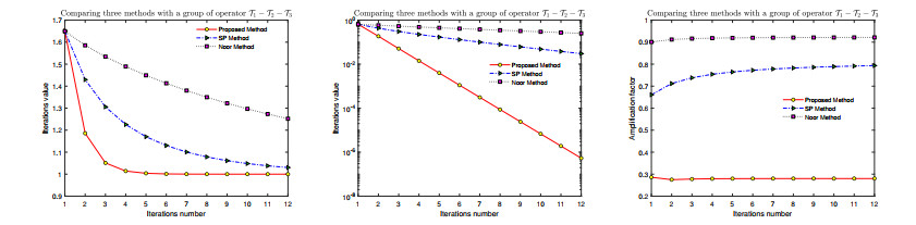
In this paper, three G-nonexpansive mappings are implemented and analyzed using an efficient modified three-step iteration algorithm. Assuming coordinate-convexity in a uniformly convex Banach space endowed with a directed graph, conditions for the weak and strong convergence of the scheme are determined. We give numerical comparisons to back up our main theorem, and compare our algorithm's convergence behavior to that of the three-step Noor iteration and SP-iteration. We use our proposed algorithm to solve image deblurring problems as an application. In addition, we discuss a novel approach to signal recovery in situations where the type of noise is unknown.
Citation: Damrongsak Yambangwai, Tanakit Thianwan. An efficient iterative algorithm for common solutions of three G-nonexpansive mappings in Banach spaces involving a graph with applications to signal and image restoration problems[J]. AIMS Mathematics, 2022, 7(1): 1366-1398. doi: 10.3934/math.2022081
In this paper, three G-nonexpansive mappings are implemented and analyzed using an efficient modified three-step iteration algorithm. Assuming coordinate-convexity in a uniformly convex Banach space endowed with a directed graph, conditions for the weak and strong convergence of the scheme are determined. We give numerical comparisons to back up our main theorem, and compare our algorithm's convergence behavior to that of the three-step Noor iteration and SP-iteration. We use our proposed algorithm to solve image deblurring problems as an application. In addition, we discuss a novel approach to signal recovery in situations where the type of noise is unknown.

| [1] |
S. Banach, Sur les oprations dans les ensembles abstraits et leur application aux quations intgrales, Fund. Math., 3 (1922), 133–181. doi: 10.4064/fm-3-1-133-181. doi: 10.4064/fm-3-1-133-181

|
| [2] |
J. Jachymski, The contraction principle for mappings on a metric space with a graph, Proc. Amer. Math. Soc., 136 (2008), 1359–1373. doi: 10.1090/S0002-9939-07-09110-1. doi: 10.1090/S0002-9939-07-09110-1
|
| [3] |
R. P. Kelisky, T. J. Rivlin, Iterates of Bernstein polynomials, Pac. J. Math., 21 (1967), 511–520. doi: 10.2140/pjm.1967.21.511. doi: 10.2140/pjm.1967.21.511
|
| [4] |
M. Samreen, T. Kamran, Fixed point theorems for integral G-contractions, Fixed Point Theory Appl., 2013 (2013), 149. doi: 10.1186/1687-1812-2013-149. doi: 10.1186/1687-1812-2013-149
|
| [5] |
J. Tiammee, S. Suantai, Coincidence point theorems for graph-preserving multivalued mappings, Fixed Point Theory Appl., 2014 (2014), 70. doi: 10.1186/1687-1812-2014-70. doi: 10.1186/1687-1812-2014-70
|
| [6] |
A. Nicolae, D. O. Regan, A. Petrusel, Fixed point theorems for single-valued and multivalued generalized contractions in metric spaces endowed with a graph, Georgian Math. J., 18 (2011), 307–327. doi: 10.1515/gmj.2011.0019. doi: 10.1515/gmj.2011.0019
|
| [7] | F. Bojor, Fixed point of $\phi$-contraction in metric spaces endowed with a graph, Ann. Univ. Craiova Mat., 37 (2010), 85–92. |
| [8] |
F. Bojor, Fixed point theorems for Reich type contractions on metric spaces with a graph, Nonlinear Anal., 75 (2012), 3895–3901. doi: 10.1016/j.na.2012.02.009. doi: 10.1016/j.na.2012.02.009
|
| [9] | F. Bojor, Fixed points of Kannan mappings in metric spaces endowed with a graph, An. St. Univ. Ovidius Constanta, 20 (2012), 31–40. |
| [10] |
J. H. Asl, B. Mohammadi, S. Rezapour, S. M. Vaezpour, Some fixed point results for generalized quasi-contractive multifunctions on graphs, Filomat, 27 (2013), 311–315. doi: 10.2298/FIL1302311A. doi: 10.2298/FIL1302311A
|
| [11] |
S. M. A. Aleomraninejad, S. Rezapour, N. Shahzad, Some fixed point result on a metric space with a graph, Topol. Appl., 159 (2012), 659–663. doi: 10.1016/j.topol.2011.10.013. doi: 10.1016/j.topol.2011.10.013
|
| [12] |
M. R. Alfuraidan, M. A. Khamsi, Fixed points of monotone nonexpansive mappings on a hyperbolic metric space with a graph, Fixed Point Theory Appl., 2015 (2015), 44. doi: 10.1186/s13663-015-0294-5. doi: 10.1186/s13663-015-0294-5
|
| [13] |
M. R. Alfuraidan, Fixed points of monotone nonexpansive mappings with a graph, Fixed Point Theory Appl., 2015 (2015), 49. doi: 10.1186/s13663-015-0299-0. doi: 10.1186/s13663-015-0299-0
|
| [14] |
J. Tiammee, A. Kaewkhao, S. Suantai, On Browder's convergence theorem and Halpern iteration process for G-nonexpansive mappings in Hilbert spaces endowed with graphs, Fixed Point Theory Appl., 2015 (2015), 187. doi: 10.1186/s13663-015-0436-9. doi: 10.1186/s13663-015-0436-9
|
| [15] |
O. Tripak, Common fixed points of G-nonexpansive mappings on Banach spaces with a graph, Fixed Point Theory Appl., 2016 (2016), 87. doi: 10.1186/s13663-016-0578-4. doi: 10.1186/s13663-016-0578-4
|
| [16] | M. A. Noor, New approximation schemes for general variational inequalities, J. Math. Anal. Appl., 251 (2000), 217–229. doi: 10.1006/jmaa.2000.7042. |
| [17] | R. Glowinski, P. L. Tallec, Augmented Lagrangian and operator-splitting methods in nonlinear mechanic, Society for Industrial and Applied Mathematics, 1989. |
| [18] |
S. Haubruge, V. H. Nguyen, J. J. Strodiot, Convergence analysis and applications of the Glowinski Le Tallec splitting method for finding a zero of the sum of two maximal monotone operators, J. Optimiz. Theory App., 97 (1998), 645–673. doi: 10.1023/a:1022646327085. doi: 10.1023/a:1022646327085
|
| [19] |
P. Sridarat, R. Suparaturatorn, S. Suantai, Y. J. Cho, Covergence analysis of SP-iteration for G-nonexpansive mappings with directed graphs, Bull. Malays. Math. Sci. Soc., 42 (2019), 2361–2380. doi: 10.1007/s40840-018-0606-0. doi: 10.1007/s40840-018-0606-0
|
| [20] | R. Johnsonbaugh, Discrete mathematics, Prentice Hall, 1997. |
| [21] |
Z. Opial, Weak convergence of the sequence of successive approximations for nonexpansive mappings, Bull. Amer. Math. Soc., 73 (1967), 591–597. doi: 10.1090/S0002-9904-1967-11761-0. doi: 10.1090/S0002-9904-1967-11761-0
|
| [22] |
S. Shahzad, R. Al-Dubiban, Approximating common fixed points of nonexpansive mappings in Banach spaces, Georgian Math. J., 13 (2006), 529–537. doi: 10.1515/GMJ.2006.529
|
| [23] |
N. V. Dung, N. T. Hieu, Convergence of a new three-step iteration process to common fixed points of three G-nonexpansivemappings in Banach spaces with directed graphs, RACSAM, 114 (2020), 140. doi: 10.1007/s13398-020-00872-w. doi: 10.1007/s13398-020-00872-w
|
| [24] |
J. Schu, Weak and strong convergence to fixed points of asymptotically nonexpansive mappings, B. Aust. Math. Soc., 43 (1991), 153–159. doi: 10.1017/S0004972700028884. doi: 10.1017/S0004972700028884
|
| [25] |
S. Suantai, Weak and strong convergence criteria of Noor iterations for asymptotically nonexpansive mappings, J. Math. Anal. Appl., 331 (2005), 506–517. doi: 10.1016/j.jmaa.2005.03.002. doi: 10.1016/j.jmaa.2005.03.002
|
| [26] |
D. Yambangwai, S. Aunruean, T. Thianwan, A new modified three-step iteration method for Gnonexpansive mappings in Banach spaces with a graph, Numer. Algor., 20 (2019), 1–29. doi: 10.1007/s11075-019-00768-w. doi: 10.1007/s11075-019-00768-w
|
| [27] |
M. G. Sangago, Convergence of iterative schemes for nonexpansive mappings, Asian-Eur. J. Math., 4 (2011), 671–682. doi: 10.1142/S1793557111000551. doi: 10.1142/S1793557111000551
|
| [28] | R. L. Burden, J. D. Faires, Numerical analysis: Cengage learning, Brooks/Cole, 2010. |
| [29] |
W. Phuengrattana, S. Suantai, On the rate of convergence of Mann, Ishikawa, Noor and SP-iterations for continuous functions on an arbitrary interval, J. Comput. Appl. Math., 235 (2011), 3006–3014. doi: 10.1016/j.cam.2010.12.022. doi: 10.1016/j.cam.2010.12.022
|
| [30] | H. H. Bauschke, P. L. Combettes, Convex analysis and monotone operator theory in Hilbert spaces, New York: Springer, 2011. |
| [31] | J. J. Moreau, Proximit$\acute{e}$ et dualit$\acute{e}$ dans un espace hilbertien, B. Soc. Math. Fr., 93 (1965), 273–299. |
| [32] |
H. F. Senter, W. G. Dotson, Approximating fixed points of nonexpansive mappings, Proc. Amer. Math. Soc., 44 (1974), 375–380. doi: 10.1090/S0002-9939-1974-0346608-8. doi: 10.1090/S0002-9939-1974-0346608-8
|


Figures(32)

Damrongsak Yambangwai, Tanakit Thianwan. An efficient iterative algorithm for common solutions of three G-nonexpansive mappings in Banach spaces involving a graph with applications to signal and image restoration problems[J]. AIMS Mathematics, 2022, 7(1): 1366-1398. doi: 10.3934/math.2022081


 DownLoad: