Comparison and application of top and bottom air decks to improve blasting operations

1.   Introduction

Fractional calculus (FC) has been increasingly garnering the interest of many mathematicians and physicians specialties in recent decades. Numerous applications of FC can be found in engineering ^[1], natural science ^[2] and many other areas. The fractional differential equations have also been effectively used to model a variety of biological issues, such as hepatitis B ^[3], methanol detoxification in the body ^[4] and the human liver ^[5], as well as other differential physics and thermodynamic models like the dynamical systems ^[6] and diffusion-wave system ^[7]. For further details, we will suggest some of the books on FC and its applications, as written by Podlubny ^[8], Samko et al. ^[9] and Kilbas et al. ^[10]. There have been various fractional derivative definitions demonstrated over the past few years. There are numerous benefits and significant implications associated with the utilization of fractional order mathematical modelling. Fractional derivatives describe a key aspect of paradigm generalization and memory consequences. Second, fractional order modelling accurately calculates details between any two points. The integer order models only cover the integer case, but fractional orders can be used at any stage. Compared to integer-order models, fractional-order models better describe memory and hereditary properties of phenomena. The Riemann-Liouville (R-L), Atangana-Baleanu-Caputo (ABC), Caputo (C), Caputo-Fabrizio (CF), Grunwald-Letnikov and Riesz derivatives are the most well-known fractional derivative definitions. The R-L and C fractional derivatives are singular kernels. The index law and other classical requirements were met by this class of fractional differential operators. This singularity prevents full physical structure memory description. Due to this constraint, Caputo and Fabrizio proposed a fractional order centered on the exponential kernel, which has a non-singular kernel ^[9,11]. Atangana Baleanu developed a non-localized derivative by using the Mittag-Leffler kernel. The CF and ABC derivative offers an alternative approach for describing FC, and it has applications in various fields. It can be used to model systems with memory and hereditary properties, and it provides a way to analyze and describe complex behaviors that cannot be fully captured by integer-order derivatives.

Researchers have started to develop various innovative ways of approximating the solution of nonlinear differential equations (NDEs) due to the difficulty of obtaining a solution to NDEs. They could be iterative approaches, perturbation methods or numerical methods. Recent years have seen several researchers working on this issue with a focus on studying fractional nonlinear partial differential equation (PDE) solutions by using a variety of techniques, including the reduced differential transform method ^[12], variational iteration method ^[13], finite difference method ^[14], iterative Laplace transform method ^[15,16] homotopy perturbation method ^[17], q-homotopy analysis transform method ^[18], finite element method ^[11], residual power series transform method ^[19], the extended sinh-Gordon equation expansion method ^[20], auxiliary equation mapping method ^[21], homotopy analysis Sumudu transform method ^[22], $(\frac{G^{\prime}}{G})$-expansion method ^[23], two-variable $(\frac{G^{\prime}}{G}, \frac{1}{G})$-expansion method ^[24], extended direct algebraic method ^[25], Hirota bilinear technique ^[26], modified Kudryashov method ^[27], symmetry group analysis ^[28,29] and so on.

The emergence of shallow-water equations (SWEs), which hold significant importance in the fields of applied mathematics and physics, can be traced back to the latter part of the 18th century. Shallow-water waves can be characterized as the observable displacements of water bodies such as the sea or ocean when subjected to physical examination. Simultaneously, numerous physical phenomena exhibiting similarities to the movements of shallow water waves are observed within the realm of various scientific disciplines, including nuclear physics, plasma physics, fluid dynamics and other related fields. Hence, the investigation of nonlinear PDEs or systems has garnered the interest of applied mathematicians in the modeling of this particular physical phenomenon. The most well-known models for shallow-water waves, according to scientific research, are based on the Klein-Gordon equation, Korteweg-de Vries equation, Benjamin-Bona-Mahony equation, Boussinesq equation, Kadomtsev-Petviashvili equation and shallow-water wave systems. The fluid must be homogeneous and incompressible, the flow must be continuous and the pressure distribution must be hydrostatic for shallow-water flows to exist. The vertical dimension must also be considerably less than the ordinary horizontal dimension. Variations of the SWEs are used to mimic a variety of geophysical flows. We consider one types of the SWEs, namely, the Benney equations ^[30], which are obtained by considering the two-dimensional and time-dependent movement of an inviscid homogeneous fluid in the presence of a gravitational field. These equations assume that the depth of the fluid is significantly smaller than the horizontal wavelengths under consideration. The equations can be expressed as follows:

where $\xi$ represents the stiff bottom and $U(\zeta, \xi, \tau)$ and $W(\zeta, \tau)$ denote the horizontal velocity component and the free surface respectively. In this context, the rigid bottom is represented by the equation $\xi = 0$, while the free surface is denoted by $\xi = W(\zeta, \tau)$. In this scenario, when the horizontal velocity component $U$ remains unaffected by changes in height $W$, Eq (1.1) simplifies to the system found in classical water theory, specifically in the context of irrotational motion. The wave motion that corresponds to this phenomenon is governed by the time-fractional coupled system of SWEs (TFCSSWE). It represents the analogous wave motion and describes a thin fluid layer in the hydrostatic equilibrium with a constant density. We consider the TFCSSWE ^[31] to be of the form

with the initial conditions

The equations under consideration in this context serve as physical models for a variety of phenomena ^[32], including tidal events, tsunamis and the hydrodynamics of lakes. Several scholars have recently explored the TFCSSWE by using various techniques, such as modified homotopy analysis transform method (MHATM), and the residual power series method (RPSM) ^[31], the homotopy perturbation method ^[33] and new iterative method (NIM) ^[34].

To the best of the authors' knowledge, this study represents the first endeavor to investigate the solutions of the TFCSSWE by utilizing the natural transform decomposition method (NTDM) while incorporating the fractional derivatives with in both singular and non-singular kernels. For a class of nonlinear PDEs, Rawashdeh and Maitama ^[35] proposed the NTDM. The Adomian decomposition method and the natural transform (NT) were two efficient techniques employed in the development of the NTDM. The proposed method handles fractional nonlinear equations without the requirement of a Lagrange multiplier, as is the case with the variational iteration method and Adomian polynomials, as well as with the Adomian decomposition method. The method under consideration does not necessitate any preconceived assumptions, linearization, perturbation or discretization, thereby mitigating the occurrence of rounding errors. As a result, the technique is ready to be applied to a wide range of nonlinear time-fractional PDEs. It is believed that this novel approach can be used to quickly and easily solve a certain class of coupled nonlinear PDEs. To acquire more insight into the impact of fractional-order derivatives, the findings were analyzed from the perspective of an infinite series. Recently, a variety of physical problems, including fractional-order concerns like the Zakharov-Kuznetsov equation ^[36], Klein-Gordon equation ^[37], coupled Kawahara and modified Kawahara equations ^[38] and Swift-Hohenberg equation ^[39], have been studied by using the proposed method.

The article's main content is presented in the following order; The primary definitions and some additional findings that are helpful in the investigation of fractional differential equations are included in Section 2. We outline the fundamental methodology for the NTDM in Section 3. The uniqueness and convergence of the solutions are examined in Section 4. The suggested strategy is put into practice in Section 5 to determine the precise solution to the TFCSSWE. The numerical results and discussion are presented in Section 6. Finally, we give our conclusions in Section 7.

2.   Basic definitions

In this section, we give some of the well-known fractional derivative definitions mentioned below.

Definition 2.1. ^[40] The C derivative of fractional order $\mu$ of function $U(\tau)\in\mathcal{C}_\nu^q$ for $\nu\ge-1$ is defined as

Definition 2.2. ^[41] The CF fractional derivative of the function $U(\tau)\in\mathbb{H}^1(0, T)$ is defined by

Definition 2.3. ^[42] The ABC derivative of fractional order $\mu$ of function $U(\tau)\in\mathbb{H}^1(0, T)$ is defined as

Definition 2.4. ^[43] The definition of the NT is given as

Definition 2.5. ^[44] The definition of the NT of the C derivative is given as

Definition 2.6. ^[45] The definition of the NT of the CF derivative is given as

where $\varphi(\mu, v, s) = 1-\mu+\mu(\frac{v}{s})$.

Definition 2.7. ^[46] The definition of the NT of the ABC derivative is given by

where $\psi(\mu, v, s) = \frac{1-\mu+\mu(\frac{v}{s})^{\mu}}{M[\mu]}$.

3.   Procedure of NTDM

In this section, the NTDM is applied to solve the TFCSSWE by considering the three aforementioned fractional derivatives.

NTDM$_{C}$: By taking the NT of Eq (1.2) in the C sense, with the initial condition given by Eq (1.3), we obtain

From Eq (3.1), we can apply the inverse NT on both sides:

The nonlinear terms can be represented as

where $A_{k}$, $B_{k}$ and $C_{k}$ are the Adomian polynomials.

$U(\zeta, \tau)$ and $W(\zeta, \tau)$ are the unknown functions, which have infinite series of the following respective forms:

Making substitutions of Eqs (3.3) and (3.4) into Eq (3.2), we obtain

From Eq (3.5), we have

Making substitutions of Eq (3.6) into Eq (3.4), we obtain the series solution as

NTDM$_{CF}$: By taking the NT of Eq (1.2) in the CF sense, with the initial condition given by Eq (1.3), we obtain

From Eq (3.8), we can apply the inverse NT on both sides:

Now, making substitutions of Eqs (3.3) and (3.4) into Eq (3.9), we have

From Eq (3.10), we have

By substituting Eq (3.11) into Eq (3.4), we obtain the series solution as

NTDM$_{ABC}$: By taking the NT of Eq (1.2), using the ABC derivative along with the initial condition given by Eq (1.3), we obtain

From Eq (3.13), we can apply the inverse NT on both sides:

Now, making substitutions of Eqs (3.3) and (3.4) into Eq (3.14), we have

From Eq (3.15), we obtain

By substituting Eq (3.16) into Eq (3.4), we obtain the series solution as

4.   Convergence analysis

The subsequent analysis will establish that the given set of sufficient conditions guarantees the existence of a unique solution. Furthermore, convergence analysis is also presented. The existence of solutions in the case of the NTDM and convergence of the solutions is established for three derivatives ^[44].

Theorem 4.1. For $0 < (\delta_1+\delta_2)\frac{\tau^\mu}{\Gamma(1+\mu)} < 1$ and $0 < (\delta_3+\delta_4)\frac{\tau^\mu}{\Gamma(1+\mu)} < 1$, the $NTDM_C$ solution is unique.

Proof. Let $H = (C[J], \left\lVert{.}\right\rVert)$ be the Banach space with $\left\lVert{\phi(\tau)}\right\rVert = \max\limits_{\tau\in J}\mid\phi(\tau)\mid$ $\forall$ continuous functions on J. Let $L:H\rightarrow H$ be a nonlinear mapping, where

Let us suppose that $\mid R_{1}(U)-R_{1}(U^*) \mid < \delta_1\mid U-U^*\mid$, $\mid F_{1}(U)-F_{1}(U^*)\mid < \delta_2\mid U-U^*\mid$ and $\mid R_{2}(W)-R_{2}(W^*) \mid < \delta_3\mid W-W^*\mid$, $\mid F_{2}(W)-F_{2}(W^*)\mid < \delta_4\mid W-W^*\mid,$ where $\delta_1$, $\delta_2$ and $\delta_3$, $\delta_4$ are Lipschitz constants and $U: = U(\zeta, \tau)$, $U^*: = U^*(\zeta, \tau)$, $W: = W(\zeta, \tau)$ and $W^*: = W^*(\zeta, \tau)$ are four different function values. Here, $F_{1}$ represents $WU_{\zeta}+UW_{\zeta}$, $R_{2}$ denotes $U_{\zeta}$ and $F_{2}$ denotes $WW_{\zeta}$.

Similarly, $\left\lVert{L_{2}(W)-L_{2}(W^*)}\right\rVert = (\delta_3+\delta_4)\frac{\tau^\mu}{\Gamma(\mu+1)}\left\lVert{W-W^*}\right\rVert$.

L is a contraction, as $0 < (\delta_1+\delta_2)\frac{\tau^\mu}{\Gamma(1+\mu)} < 1$ and $0 < (\delta_3+\delta_4)\frac{\tau^\mu}{\Gamma(1+\mu)} < 1$. From the perspective of the Banach fixed-point theorem, the solution is unique. □

Using procedure similar to Theorem 4.1, we state the following.

Theorem 4.2. The $NTDM_{CF}$ solution is unique when $0 < (\delta_1 +\delta_2)(1-\mu +\mu \tau) < 1$ and $0 < (\delta_3 +\delta_4)(1-\mu +\mu \tau) < 1$.

Theorem 4.3. The $NTDM_{ABC}$ solution is unique when $0 < (\delta_1 +\delta_2)(1-\mu +\mu \frac{\tau^\mu}{\Gamma(\mu+1)}) < 1$ and $0 < (\delta_3 +\delta_4)(1-\mu +\mu \frac{\tau^\mu}{\Gamma(\mu+1)}) < 1$.

Theorem 4.4. The $NTDM_C$ solution is convergent.

Proof. Let $U_m = \sum\limits _{k = 0}^{m}U_k(\zeta, \tau)$ and $W_m = \sum\limits _{k = 0}^{m}W_k(\zeta, \tau)$. To prove that $U_m$ and $W_m$ are Cauchy sequences in $H$, consider the following:

Similarly, $\left\lVert{W_m-W_n}\right\rVert = (\delta_3+\delta_4)\frac{\tau^\mu}{\Gamma(\mu+1)}\left\lVert{W_{m-1}-W_{n-1}}\right\rVert$.

Let $m = n+1$ ; then,

Similarly, $\left\lVert{W_{n+1}-W_n}\right\rVert\leq\rho^n\left\lVert{W_1-W_0}\right\rVert$, where $\delta = (\delta_1+\delta_2)\frac{\tau^\mu}{\Gamma(\mu+1)}$ and $\rho = (\delta_3+\delta_4)\frac{\tau^\mu}{\Gamma(\mu+1)}$. Moreover, we have

Similarly, $\left\lVert{W_m-W_n}\right\rVert\leq\rho^n\Big(\frac{1-\rho^{m-n}}{1-\rho}\Big)\left\lVert{W_1}\right\rVert$.

Because $0 < \delta < 1$ and $0 < \rho < 1$, we get that $1-\delta^{m-n} < 1$ and $1-\rho^{m-n} < 1$.

Therefore, $\left\lVert{U_m-U_n}\right\rVert\leq\frac{\delta^{n}}{1-\delta} \max_{\tau\in J}\left\lVert{U_1}\right\rVert$ and $\left\lVert{W_m-W_n}\right\rVert\leq\frac{\rho^{n}}{1-\rho} \max_{\tau\in J}\left\lVert{W_1}\right\rVert$.

Since $\left\lVert{U_1}\right\rVert < \infty$ and $\left\lVert{W_1}\right\rVert < \infty$ results in $n\rightarrow \infty$, $\left\lVert{U_m-U_n}\right\rVert\rightarrow 0$ and $\left\lVert{W_m-W_n}\right\rVert\rightarrow 0$. As a result, $U_m$ and $W_{m}$ are Cauchy sequences in H; thus, the series $U_m$ and $W_{m}$ are convergent. □

Using a procedure similar to Theorem 4.4, we state the following:

Theorem 4.5. The $NTDM_{CF}$ solution is convergent.

Theorem 4.6. The $NTDM_{ABC}$ solution is convergent.

5.   Numerical example of TFCSSWE

In this section, the approximate solutions of the TFCSSWE , as obtained by applying three fractional derivatives namely, the C, CF and ABC derivatives, are presented.

Consider the TFCSSWE given by Eq (1.2), along with the initial conditions given by Eq (1.3), and when $\mu = 1$, the exact solution ^[31] is given by

NTDM$_{C}$: We get the NTDM$_{C}$ solutions as follows:

Similar expressions for ${}^{C}U_{k}(\zeta, \tau)$ and ${}^{C}W_{k}(\zeta, \tau)$ for $k \ge 4$ can also be obtained by using Eq (3.6). We get the series solution from Eq (3.7) as follows:

NTDM$_{CF}$: We get the NTDM$_{CF}$ solutions as follows:

Similar expressions for ${}^{CF}U_{k}(\zeta, \tau)$ and ${}^{CF}W_{k}(\zeta, \tau)$ for $k \ge 4$ can also be obtained by using Eq (3.11). We get the series solution from Eq (3.12) as follows:

NTDM$_{ABC}$: We get the NTDM$_{ABC}$ solutions as follows:

Similar expressions for ${}^{ABC}U_{k}(\zeta, \tau)$ and ${}^{ABC}W_{k}(\zeta, \tau)$ for $k \ge 4$ can also be obtained by using Eq (3.16). We get the series solution from Eq (3.17) as follows:

6.   Numerical results and discussion

In this section, we present the numerical and graphical simulations of the TFCSSWE by using the NTDM. The solutions were computed by using distinct spatial and temporal variables for different fractional-order values, as shown in Tables 1–6. Figures 1–4 present the results of numerical simulations that exploit the animations of the solutions, showcasing their dynamic behavior. Tables 1–4 present the absolute error of the TFCSSWE for different values of $\zeta$ and $\tau$, with $\mu$ set to 1. Tables 1 and 2 present a comparative analysis of the absolute errors associated with the horizontal velocity $U(\zeta, \tau)$ and free surface $W(\zeta, \tau)$, as conducted by employing MHATM and RPSM methodologies ^[31]. Tables 3 and 4 present a comparative analysis of the absolute errors of $U$ and $W$, as based on the NIM ^[34].

Based on the data presented in Tables 1–4, it is evident that the suggested method solutions for all three derivatives exhibit high levels of concordance with the approaches that have been reported in the literature. The provided test example showcases the efficacy, adaptability and accuracy of the proposed methodology. This observation illustrates that the proposed numerical method yields more favorable outcomes when applied to NDEs. After successfully validating the strategy for the integer-order model, the authors were motivated to apply the recommended method to solve the comparable model, i.e., a temporal fractional-order model. Table 5 demonstrates that the behavior of the horizontal velocity derived from both singular and non-singular kernel derivatives exhibits a further significant increase when the fractional order decreases. Table 6 illustrates the observed behavior of the free surface as derived from both singular and non-singular kernel derivatives, we can observe substantial decreases as the fractional order decreases.

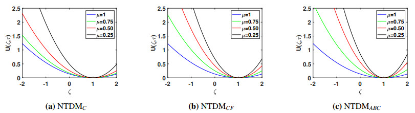
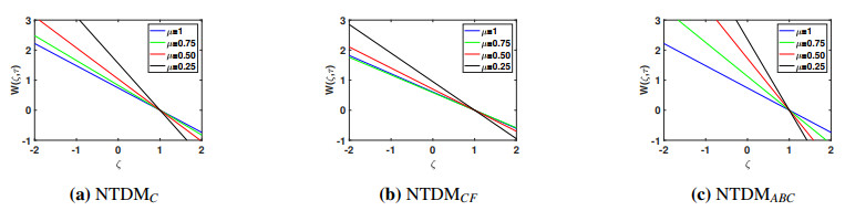
In Figures 1 and 2, the graphical representations respectively showcase the estimated solutions $U(\zeta, \tau)$ and $W(\zeta, \tau)$ for $\mu = 0.25, 0.50, 0.75, 1$, $0\le\zeta\le5$ when $\tau$ is set to 0.1. As the value of $\zeta$ increases and the fractional order decreases, Figure 1 illustrates that the horizontal velocity component $U(\zeta, \tau)$ increases under the condition of a constant $\tau$. According to Figure 2, as the value of $\zeta$ increases and the fractional order decreases, the free surface $W(\zeta, \tau)$ experiences a drop while keeping $\tau$ constant.

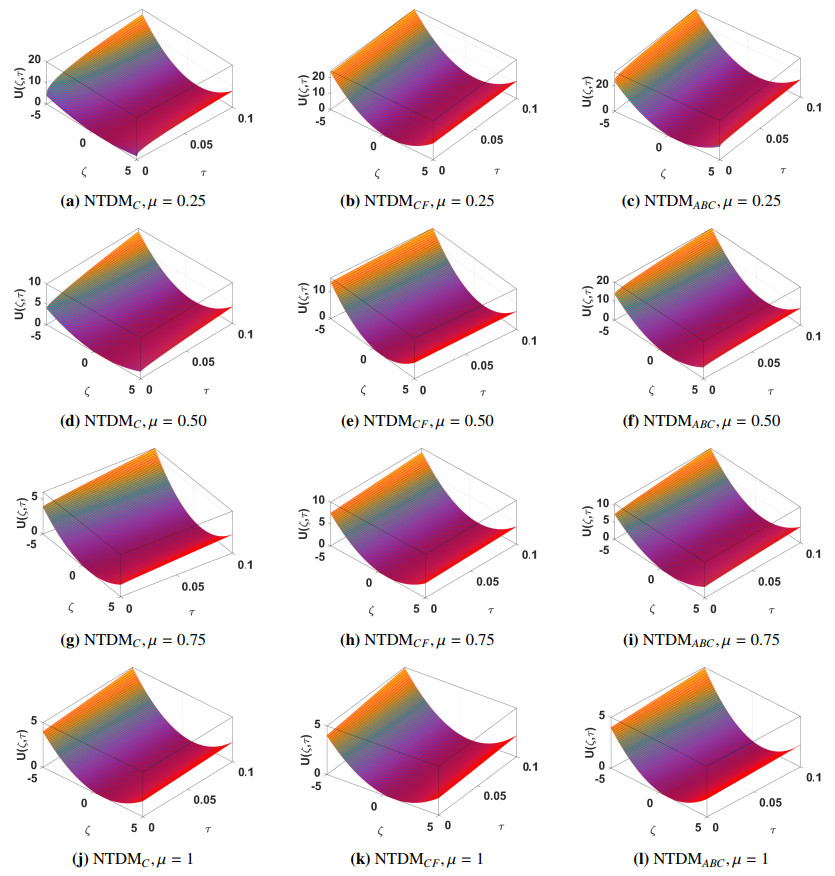
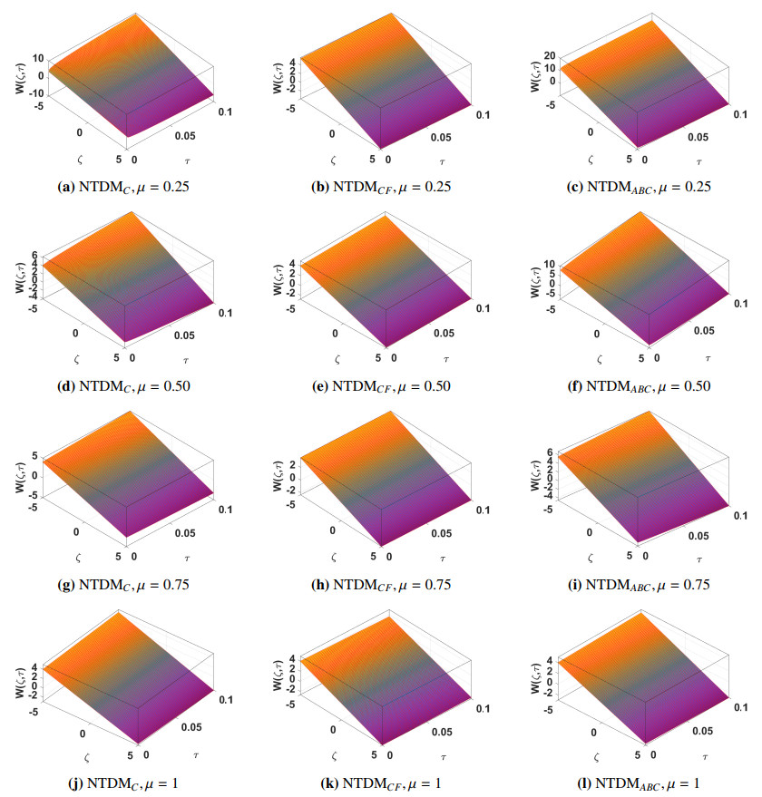
Figures 3 and 4 respectively provide surface plots of the horizontal velocity component $U(\zeta, \tau)$ and the free surface $W(\zeta, \tau)$ for $\mu = 0.25, 0.50, 0.75, 1$, $-5\le\zeta\le5$ and $0\le\tau\le 0.1$. Based on the data shown in the tables and figures, it can be noticed that there is a strong level of concurrence among all three derivatives. The methodology outlined in this paper elucidates that when the fractional order approaches the classical scenario, the obtained solution likewise converges toward the analytical solution. This finding serves to validate the accuracy of the used scheme. Hence, the tangible manifestation of our findings can potentially serve as a valuable instrument for exploring additional discoveries pertaining to nonlinear wave phenomena in scientific applications.

7.   Conclusions

We applied the NTDM approach to study the horizontal velocity and free surface of a TFCSSWE arising in ocean engineering. The fractional derivative has been applied from the perspectives of the C, CF and ABC approaches. The analytical solutions derived by using the NTDM approach, according to the results, are relatively close to the precise solutions. According to the tables and graphs, the approximate solution of the differential equation converges to the exact solution when $\mu = 1$. The technique presented in this study showcases the validity and efficacy of the implemented method through a comparative analysis of the obtained results with those reported in previous studies. Thus, the proposed approach for obtaining numerical and analytical solutions to nonlinear problems is exceptionally trustworthy and efficient. The subsequent findings illustrate that the suggested methodology is exceptionally effective. The aforementioned methodology exhibits reliability, straightforwardness and innovation in its application to the resolution of fractional- order systems of differential equations. Our findings are expected to make a valuable contribution to future research on the behavior of SWEs in various fields, including mathematical physics, applied mathematics, ocean engineering, civil engineering and port and coastal construction. Further, this method can be used to analyze nonlinear fractional-order mathematical models of infectious diseases like Ebola, hepatitis, tuberculosis and others.

Use of AI tools declaration

The authors declare that they have not used artificial Intelligence tools in the creation of this article.

Acknowledgements

The authors would like to thank the reviewers for their thorough reading and insightful comments, observations and suggestions that significantly improved the manuscript.

Conflict of interest

The authors declare no conflicts of interest.