Nonlinear analysis of a nonlinear modified KdV equation under Atangana Baleanu Caputo derivative

Gulalai; Shabir Ahmad; Fathalla Ali Rihan; Aman Ullah; Qasem M. Al-Mdallal; Ali Akgül; Gulalai; Shabir Ahmad; Fathalla Ali Rihan; Aman Ullah; Qasem M. Al-Mdallal; Ali Akgül

doi:10.3934/math.2022439

AIMS Mathematics

2022, Volume 7, Issue 5: 7847-7865. doi: 10.3934/math.2022439

Previous Article Next Article

Research article Special Issues

Nonlinear analysis of a nonlinear modified KdV equation under Atangana Baleanu Caputo derivative

1.
Department of Mathematics, University of Malakand, Dir(L), Khyber Pakhtunkhwa, Pakistan
2.
Department of Mathematical Sciences, United Arab Emirates University, P.O. Box 15551, Al Ain, Abu Dhabi, UAE
3.
Art and Science Faculty, Department of Mathematics, Siirt University, TR-56100 Siirt, Turkey

Received: 13 September 2021 Revised: 27 October 2021 Accepted: 28 October 2021 Published: 17 February 2022
MSC : 35R11

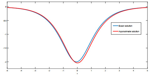
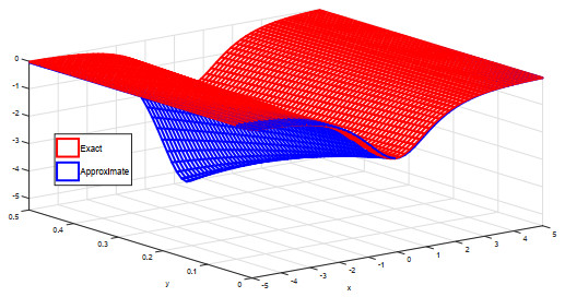
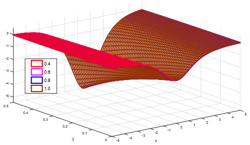
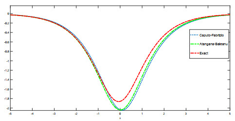
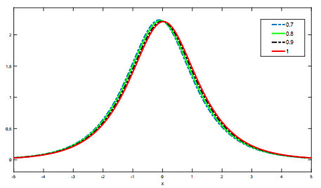
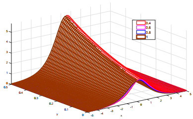
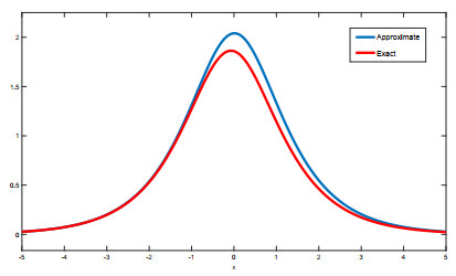
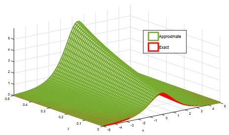
The focus of the current manuscript is to provide a theoretical and computational analysis of the new nonlinear time-fractional (2+1)-dimensional modified KdV equation involving the Atangana-Baleanu Caputo ($ \mathcal{ABC} $) derivative. A systematic and convergent technique known as the Laplace Adomian decomposition method (LADM) is applied to extract a semi-analytical solution for the considered equation. The notion of fixed point theory is used for the derivation of the results related to the existence of at least one and unique solution of the mKdV equation involving under $ \mathcal{ABC} $-derivative. The theorems of fixed point theory are also used to derive results regarding to the convergence and Picard's X-stability of the proposed computational method. A proper investigation is conducted through graphical representation of the achieved solution to determine that the $ \mathcal{ABC} $ operator produces better dynamics of the obtained analytic soliton solution. Finally, 2D and 3D graphs are used to compare the exact solution and approximate solution. Also, a comparison between the exact solution, solution under Caputo-Fabrizio, and solution under the $ \mathcal{ABC} $ operator of the proposed equation is provided through graphs, which reflect that $ \mathcal{ABC} $-operator produces better dynamics of the proposed equation than the Caputo-Fabrizio one.
- Atangana-Baleanu fractional operator,
- fixed point theory,
- Laplace Adomian decomposition
Citation: Gulalai, Shabir Ahmad, Fathalla Ali Rihan, Aman Ullah, Qasem M. Al-Mdallal, Ali Akgül. Nonlinear analysis of a nonlinear modified KdV equation under Atangana Baleanu Caputo derivative[J]. AIMS Mathematics, 2022, 7(5): 7847-7865. doi: 10.3934/math.2022439

Related Papers:

Abstract

The focus of the current manuscript is to provide a theoretical and computational analysis of the new nonlinear time-fractional (2+1)-dimensional modified KdV equation involving the Atangana-Baleanu Caputo ($ \mathcal{ABC} $) derivative. A systematic and convergent technique known as the Laplace Adomian decomposition method (LADM) is applied to extract a semi-analytical solution for the considered equation. The notion of fixed point theory is used for the derivation of the results related to the existence of at least one and unique solution of the mKdV equation involving under $ \mathcal{ABC} $-derivative. The theorems of fixed point theory are also used to derive results regarding to the convergence and Picard's X-stability of the proposed computational method. A proper investigation is conducted through graphical representation of the achieved solution to determine that the $ \mathcal{ABC} $ operator produces better dynamics of the obtained analytic soliton solution. Finally, 2D and 3D graphs are used to compare the exact solution and approximate solution. Also, a comparison between the exact solution, solution under Caputo-Fabrizio, and solution under the $ \mathcal{ABC} $ operator of the proposed equation is provided through graphs, which reflect that $ \mathcal{ABC} $-operator produces better dynamics of the proposed equation than the Caputo-Fabrizio one.

References

[1]	Korteweg-De Vries equation, Wikipedia. Available from: https://en.wikipedia.org/wiki/Korteweg-de_Vries_equation.
[2]	A. M. Wazwaz, New sets of solitary wave solutions to the KdV, mKdV, and the generalized KdV equations, Commun. Nonlinear Sci. Numer. Simul., 13 (2008), 331–339. https://doi.org/10.1016/j.cnsns.2006.03.013 doi: 10.1016/j.cnsns.2006.03.013
[3]	C. Wang, Spatiotemporal deformation of lump solution to (2+1)-dimensional KdV equation, Nonlinear Dyn., 84 (2016), 697–702. https://doi.org/10.1007/s11071-015-2519-x doi: 10.1007/s11071-015-2519-x
[4]	B. R. Sontakke, A. Shaikh, The new iterative method for approximate solutions of time fractional KdV, K(2, 2), Burgers and cubic Boussinesq equations, Asian Res. J. Math., 1 (2016), 1–10.
[5]	Y. Shi, B. Xu, Y. Guo, Numerical solution of Korteweg-de Vries-Burgers equation by the compact-type CIP method, Adv. Differ. Equ., 2015 (2015), 353. https://doi.org/10.1186/s13662-015-0682-5 doi: 10.1186/s13662-015-0682-5
[6]	A. R. Seadawy, New exact solutions for the KdV equation with higher order nonlinearity by using the variational method, Comput. Math. Appl., 62 (2011), 3741–3755. https://doi.org/10.1016/j.camwa.2011.09.023 doi: 10.1016/j.camwa.2011.09.023
[7]	G. Wang, A. H. Kara, A (2+1)-dimensional KdV equation and mKdV equation: Symmetries, group invariant solutions and conservation laws, Phys. Lett. A, 383 (2019), 728–731. https://doi.org/10.1016/j.physleta.2018.11.040 doi: 10.1016/j.physleta.2018.11.040
[8]	M. G. Sakar, A. Akgül, D. Baleanu, On solutions of fractional Riccati differential equations, Adv. Differ. Equ., 2017 (2017), 1–10. https://doi.org/10.1186/s13662-017-1091-8 doi: 10.1186/s13662-017-1091-8
[9]	M. D. Ikram, M. I. Asjad, A. Akgül, D. Baleanu, Effects of hybrid nanofluid on novel fractional model of heat transfer flow between two parallel plates, Alexandria Eng. J., 60 (2021), 3593–3604. https://doi.org/10.1016/j.aej.2021.01.054 doi: 10.1016/j.aej.2021.01.054
[10]	A. Akgül, D. Baleanu, On solutions of variable-order fractional differential equations, Int. J. Optim. Control: Theor. Appl., 7 (2017), 112–116. https://doi.org/10.11121/ijocta.01.2017.00368 doi: 10.11121/ijocta.01.2017.00368
[11]	M. Caputo, M. Fabrizio, A new definition of fractional derivative without singular kernel, Progr. Fract. Differ. Appl., 1 (2015), 1–13.
[12]	A. Atangana, D. Baleanu, New fractional derivatives with non-local and nonsingular kernel: Theory and application to heat transfer model, Therm. Sci., 20 (2016), 763–769. https://doi.org/10.2298/TSCI160111018A doi: 10.2298/TSCI160111018A
[13]	S. Bushnaq, K. Shah, H. Alrabaiah, On modeling of coronavirus-19 disease under Mittag-Leffler power law, Adv. Differ. Equ., 2020 (2020), 487. https://doi.org/10.1186/s13662-020-02943-z doi: 10.1186/s13662-020-02943-z
[14]	S. Ahmad, A. Ullah, A. Akgül, D. Baleanu, Analysis of the fractional tumour-immune-vitamins model with Mittag-Leffler kernel, Results Phys., 19 (2020), 103559. https://doi.org/10.1016/j.rinp.2020.103559 doi: 10.1016/j.rinp.2020.103559
[15]	S. Ahmad, A. Ullah, M. Arfan, K. Shah, On analysis of the fractional mathematical model of rotavirus epidemic with the effects of breastfeeding and vaccination under Atangana-Baleanu (AB) derivative, Chaos Solitons Fractals, 140, (2020), 110233. https://doi.org/10.1016/j.chaos.2020.110233 doi: 10.1016/j.chaos.2020.110233
[16]	M. Yavuz, N. Ozdemir, H. M. Baskonus, Solutions of partial differential equations using the fractional operator involving Mittag-Leffler kernel, Eur. Phys. J. Plus, 133 (2018), 215. https://doi.org/10.1140/epjp/i2018-12051-9 doi: 10.1140/epjp/i2018-12051-9
[17]	M. A. Taneco-Hernández, V. F. Morales-Delgado, J. F. Gómez-Aguilar, Fractional Kuramoto-Sivashinsky equation with power law and stretched Mittag-Leffler kernel, Phys. A: Stat. Mech. Appl., 527 (2019), 121085. https://doi.org/10.1016/j.physa.2019.121085 doi: 10.1016/j.physa.2019.121085
[18]	D. Baleanu, B. Shiri, H. M. Srivastava, M. Al Qurashi, A Chebyshev spectral method based on operational matrix for fractional differential equations involving non-singular Mittag-Leffler kernel, Adv. Differ. Equ., 2018 (2018), 353. https://doi.org/10.1186/s13662-018-1822-5 doi: 10.1186/s13662-018-1822-5
[19]	A. Saadatmandi, M. Dehghan, A new operational matrix for solving fractional-order differential equations, Comput. Math. Appl., 59 (2010), 1326–1336. https://doi.org/10.1016/j.camwa.2009.07.006 doi: 10.1016/j.camwa.2009.07.006
[20]	X. Zhang, L. Juan, An analytic study on time-fractional Fisher equation using homotopy perturbation method, Walailak J. Sci. Tech., 11 (2014), 975–985. http://dx.doi.org/10.14456/WJST.2014.72 doi: 10.14456/WJST.2014.72
[21]	D. Baleanu, H. K. Jassim, Exact solution of two-dimensional fractional partial differential equations, Fractal Fract., 4 (2020), 21. https://doi.org/10.3390/fractalfract4020021 doi: 10.3390/fractalfract4020021
[22]	S. Ahmad, A. Ullah, K. Shah, A. Akgül, Computational analysis of the third order dispersive fractional PDE under exponential-decay and Mittag-Leffler type kernels, Numer. Methods Partial Differ. Equ., 2020, 1–16. https://doi.org/10.1002/num.22627
[23]	H. Jafari, C. M. Khalique, M. Nazari, Application of the Laplace decomposition method for solving linear and nonlinear fractional diffusion-wave equations, Appl. Math. Lett., 24 (2011), 1799–1805. https://doi.org/10.1016/j.aml.2011.04.037 doi: 10.1016/j.aml.2011.04.037
[24]	F. Haq, K. Shah, G. Ur-Rahman, M. Shahzad, Numerical solution of fractional order smoking model via Laplace Adomian decomposition method, Alexandria Eng. J., 57 (2018), 1061–1069. https://doi.org/10.1016/j.aej.2017.02.015 doi: 10.1016/j.aej.2017.02.015
[25]	Y. Qing, B. E. Thoades, $T$-stability on picard iteration in metric space, Fixed Point Theory Appl., 2008 (2008), 418971. https://doi.org/10.1155/2008/418971 doi: 10.1155/2008/418971

Reader Comments

Your name:*

Email:*
© 2022 the Author(s), licensee AIMS Press. This is an open access article distributed under the terms of the Creative Commons Attribution License (http://creativecommons.org/licenses/by/4.0)