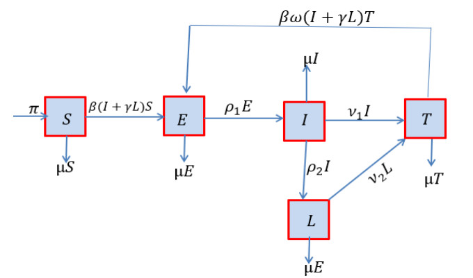
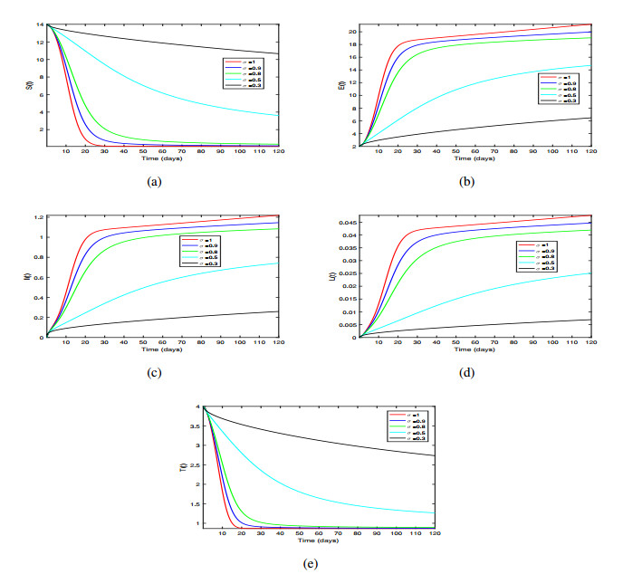
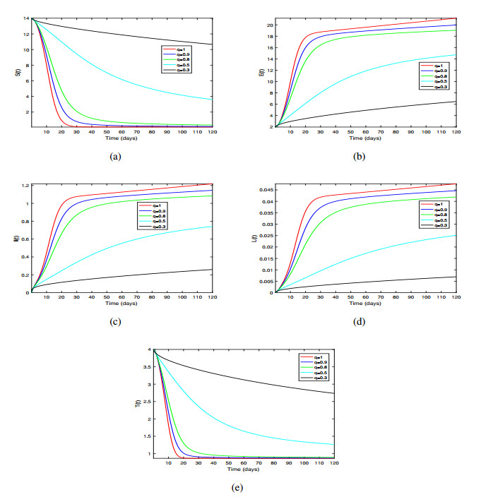
Syphilis is one the most dangerous sexually transmitted disease which is common in the world. In this work, we formulate and analyze a mathematical model of Syphilis with an emphasis on treatment in the sense of Caputo-Fabrizio (CF) and Atangana-Baleanu (Mittag-Leffler law) derivatives. The basic reproduction number of the CF model which presents information on the spread of the disease is determined. The model's steady states were found, and the disease-free state's local and global stability are established based on the basic reproduction number. The existence and uniqueness of solutions for both Caputo-Fabrizio and Atangana-Baleanu derivative in the Caputo sense are established. Numerical simulations were carried out to support the analytical solution, which indicates that the fractional-order derivatives influence the dynamics of the spread of Syphilis in any community induced with the disease.
Citation: E. Bonyah, C. W. Chukwu, M. L. Juga, Fatmawati. Modeling fractional-order dynamics of Syphilis via Mittag-Leffler law[J]. AIMS Mathematics, 2021, 6(8): 8367-8389. doi: 10.3934/math.2021485
Syphilis is one the most dangerous sexually transmitted disease which is common in the world. In this work, we formulate and analyze a mathematical model of Syphilis with an emphasis on treatment in the sense of Caputo-Fabrizio (CF) and Atangana-Baleanu (Mittag-Leffler law) derivatives. The basic reproduction number of the CF model which presents information on the spread of the disease is determined. The model's steady states were found, and the disease-free state's local and global stability are established based on the basic reproduction number. The existence and uniqueness of solutions for both Caputo-Fabrizio and Atangana-Baleanu derivative in the Caputo sense are established. Numerical simulations were carried out to support the analytical solution, which indicates that the fractional-order derivatives influence the dynamics of the spread of Syphilis in any community induced with the disease.

| [1] |
Z. Q. Chen, G. C. Zhang, X. D. Gong, C. Lin, X. Gao, G. J. Liang, Syphilis in China: results of a national surveillance programme, The Lancet, 369 (2007), 132–138. doi: 10.1016/S0140-6736(07)60074-9

|
| [2] |
L. Doherty, K. A. Fenton, J. Jones, T. C. Paine, S. P. Higgins, D. Williams, et al. Syphilis: old problem, new strategy, BMJ, 325 (2002), 153–156. doi: 10.1136/bmj.325.7356.153
|
| [3] | CDC, Sexually transmitted diseases. Centers for disease control and prevention, 20 January 2010. Available from: https://www.cdc.gov/std/syphilis/stdfact-syphilis-detailed.htm: :text=Syphilis%20is%20transmitted%20from%20person,%2C%20anal%2C%20or%20oral%20sex. |
| [4] | D. Aadland, D. C. Finnoff, K. X. Huang, Syphilis cycles, BE J. Economic Anal. Policy, 14 (2013), 297–348. |
| [5] |
G. P. Garnett, S. O. Aral, D. V. Hoyle, W. Cates, R. M. Anderson, The natural history of syphilis: Implications for the transmission dynamics and control of infection, Sex. Transm. Dis., 24 (1997), 185–200. doi: 10.1097/00007435-199704000-00002
|
| [6] |
M. Myint, H. Bashiri, R. D. Harrington, C. M. Marra, Relapse of secondary syphilis after benzathine penicillin G: molecular analysis, Sex. Trans. Dis., 31 (2004), 196–199. doi: 10.1097/01.OLQ.0000114941.37942.4C
|
| [7] | N. R. Birnbaum, R. H. Goldschmidt, W. Buffet, Resolving the common clinical dilemmas of syphilis, Am. Fam. Physician, 59 (1999), 2233. |
| [8] | M. L. Juga, F. Nyabadza, Modelling the Ebola virus disease dynamics in the presence of interfered interventions, Commun. Math. Biol. Neurosci., 2020 (2020), 1–30. |
| [9] | C. W. Chukwu, J. Mushanyu, M. L. Juga, Fatmawati, A mathematical model for co-dynamics of Listeriosis and bacterial meningitis diseases, Commun. Math. Biol. Neurosci., 2020 (2020), 1–20. |
| [10] | E. Bonyah, M. Juga, W. Chukwu, Fatmawati, A fractional order dengue fever model in the context of protected travellers, Available from: https://www.medrxiv.org/content/10.1101/2021.01.09.21249522v1, 2021. |
| [11] | C. W. Chukwu, F. Nyabadza, A mathematical model and optimal control for Listeriosis disease from ready-to-eat food products, Available from: https://www.medrxiv.org/content/10.1101/2020.10.11.20210856v1, 2020. |
| [12] | C. W. Chukwu, F. Nyabadza, A theoretical model of Listeriosis driven by cross contamination of ready-to-eat food products, Int. J. Math. Math. Sci., 2020, (2020). |
| [13] |
Fatmawati, D. U. Purwati, F. Riyudha, H. Tasman, Optimal control of a discrete age-structured model for tuberculosis transmission, Heliyon, 6 (2020), e03030. doi: 10.1016/j.heliyon.2019.e03030
|
| [14] |
B. Pourbohloul, M. L. Rekart, R. C. Brunham, Impact of mass treatment on syphilis transmission: A mathematical modeling approach, J. Sex. Transm. Dis., 30 (2003), 297–305. doi: 10.1097/00007435-200304000-00005
|
| [15] | F. Milner, R. Zhao, A new mathematical model of syphilis, J. Sex. Transm. Dis., 5 (2010), 96-–108. |
| [16] |
E. Iboi, D. Okuonghae, Population dynamics of a mathematical model for syphilis, Appl. Math. Model., 40 (2016), 3573–3590. doi: 10.1016/j.apm.2015.09.090
|
| [17] | M. Caputo, M. Fabrizio, A new definition of fractional derivative without singular kernel, Progr. Fract. Diff. Appl., 1 (2015), 1–13. |
| [18] | A. Atangana, D. Baleanu, New fractional derivatives with nonlocal and non-singular kernel: Theory and application to heat transfer model, Therm. Sci., 20 (2016). |
| [19] |
A. Atangana, I. Koca, Chaos in a simple nonlinear system with Atangana–Baleanu derivatives with fractional order, Chaos, Solitons Fractals, 89 (2016), 447–454. doi: 10.1016/j.chaos.2016.02.012
|
| [20] |
M. A. Khan, S. Ullah, M. Farooq, A new fractional model for tuberculosis with relapse via Atangana–Baleanu derivative, Chaos, Solitons Fractals, 116 (2018), 227–238. doi: 10.1016/j.chaos.2018.09.039
|
| [21] |
E. Bonyah, Chaos in a 5-D hyperchaotic system with four wings in the light of non-local and non-singular fractional derivatives, Chaos, Solitons Fractals, 116 (2018), 316–331. doi: 10.1016/j.chaos.2018.09.034
|
| [22] |
A. Akgül, A novel method for a fractional derivative with non-local and non-singular kernel, Chaos, Solitons Fractals, 114 (2018), 478–482. doi: 10.1016/j.chaos.2018.07.032
|
| [23] | A. Akgül, Analysis and new applications of fractal fractional differential equations with power law kernel, Discrete Continuous Dyn. Syst. Ser. S, 116 (2020). Available from: doi:10.3934/dcdss.2020423. |
| [24] |
A. Akgül, E. K. Akgül, A novel method for solutions of fourth-order fractional boundary value problems, Fract. Fraction., 3 (2019), 1–13. doi: 10.3390/fractalfract3010001
|
| [25] | E. K. Akgül, A. Akgül, D. Baleanu, Laplace transform method for economic models with constant proportional Caputo derivative, Fractal Fractional, 4 (2020), 1–10. |
| [26] |
A. Akgül, D. Baleanu, Analysis and applications of the proportional Caputo derivative, Adv. Differ. Eq., 2021 (2021), 136. doi: 10.1186/s13662-021-03304-0
|
| [27] |
Fatmawati, M. A. Khan, E. Bonyah, Z. Hammouch, E. M. Shaiful, A mathematical model of tuberculosis (TB) transmission with children and adults groups: A fractional model, AIMS Mathematics, 5 (2020), 2813–2842. doi: 10.3934/math.2020181
|
| [28] | J. Losada, J. J. Nieto, Properties of a new fractional derivative without singular kernel, Progr. Fract. Diff. Appl., 1 (2015), 87–92. |
| [29] | Z. M. Odibat, N. T. Shawagfeh, Generalized Taylor's formula, Appl. Math. Comput., 186 (2007), 286–293. |
| [30] |
P. van den Driessche, J. Watmough, Reproduction numbers and sub-threshold endemic equilibria for compartmental models of disease transmission, Math. Biosci., 180 (2002), 29–48. doi: 10.1016/S0025-5564(02)00108-6
|
| [31] | J. La Salle, S. Lefschetz, R. Alverson, Stability by Liapunov's direct method with applications, Phys. Today, 15 (1962), 59. |
| [32] |
A. Atangana, K. M. Owolabi, New numerical approach for fractional differential equations, Math. Model. Nat. Phenom., 13 (2018), 3. doi: 10.1051/mmnp/2018010
|
| [33] | S. Ullah, M. A. Khan, M. Farooq, Z. Hammouch, D. Baleanu, A fractional model for the dynamics of tuberculosis infection using Caputo-Fabrizio derivative, Discrete Continuous Dyn. Syst. Ser. S, 13 (2020), 975. |
| [34] |
A. Atangana, E. Bonyah, A. Elsadany, A fractional order optimal 4D chaotic financial model with Mittag-Leffler law, Chinese J. Phys., 65 (2020), 38–53. doi: 10.1016/j.cjph.2020.02.003
|
| [35] |
M. Toufik, A. Atangana, New numerical approximation of fractional derivative with non-local and non-singular kernel: Application to chaotic models, Eur. Phys. J. Plus, 132 (2017), 444. doi: 10.1140/epjp/i2017-11717-0
|
Figures(3)

E. Bonyah, C. W. Chukwu, M. L. Juga, Fatmawati. Modeling fractional-order dynamics of Syphilis via Mittag-Leffler law[J]. AIMS Mathematics, 2021, 6(8): 8367-8389. doi: 10.3934/math.2021485


 DownLoad: