
A previously unknown relationship between the tidal forces and aa index is shown and used to discuss when the next maximum of the annual aa index is expected to occur.
Citation: Mikhail Kovalyov. On the relationship between the aa index and tidal forces[J]. AIMS Geosciences, 2021, 7(4): 582-588. doi: 10.3934/geosci.2021034
[1] | Ahmed Alamer, Hassan Zafar, Muhammad Javaid . Study of modified prism networks via fractional metric dimension. AIMS Mathematics, 2023, 8(5): 10864-10886. doi: 10.3934/math.2023551 |
[2] | Pradeep Singh, Sahil Sharma, Sunny Kumar Sharma, Vijay Kumar Bhat . Metric dimension and edge metric dimension of windmill graphs. AIMS Mathematics, 2021, 6(9): 9138-9153. doi: 10.3934/math.2021531 |
[3] | Mohra Zayed, Ali Ahmad, Muhammad Faisal Nadeem, Muhammad Azeem . The comparative study of resolving parameters for a family of ladder networks. AIMS Mathematics, 2022, 7(9): 16569-16589. doi: 10.3934/math.2022908 |
[4] | Chenggang Huo, Humera Bashir, Zohaib Zahid, Yu Ming Chu . On the 2-metric resolvability of graphs. AIMS Mathematics, 2020, 5(6): 6609-6619. doi: 10.3934/math.2020425 |
[5] | Meiqin Wei, Jun Yue, Xiaoyu zhu . On the edge metric dimension of graphs. AIMS Mathematics, 2020, 5(5): 4459-4465. doi: 10.3934/math.2020286 |
[6] | Yuni Listiana, Liliek Susilowati, Slamin Slamin, Fadekemi Janet Osaye . A central local metric dimension on acyclic and grid graph. AIMS Mathematics, 2023, 8(9): 21298-21311. doi: 10.3934/math.20231085 |
[7] | Chunqiang Cui, Jin Chen, Shixun Lin . Metric and strong metric dimension in TI-power graphs of finite groups. AIMS Mathematics, 2025, 10(1): 705-720. doi: 10.3934/math.2025032 |
[8] | Syed Ahtsham Ul Haq Bokhary, Zill-e-Shams, Abdul Ghaffar, Kottakkaran Sooppy Nisar . On the metric basis in wheels with consecutive missing spokes. AIMS Mathematics, 2020, 5(6): 6221-6232. doi: 10.3934/math.2020400 |
[9] | Xiaogang Liu, Muhammad Ahsan, Zohaib Zahid, Shuili Ren . Fault-tolerant edge metric dimension of certain families of graphs. AIMS Mathematics, 2021, 6(2): 1140-1152. doi: 10.3934/math.2021069 |
[10] | Ahmet Sinan Cevik, Ismail Naci Cangul, Yilun Shang . Matching some graph dimensions with special generating functions. AIMS Mathematics, 2025, 10(4): 8446-8467. doi: 10.3934/math.2025389 |
A previously unknown relationship between the tidal forces and aa index is shown and used to discuss when the next maximum of the annual aa index is expected to occur.
In the last few years, it has been proved that Brauer configuration algebras (BCAs) are a helpful tool in different fields of applied mathematics [1,2,3]. In particular, they were used in cryptography and the theory of graph energy. Green and Schroll introduced such algebras as a generalization of Brauer graph algebras. Bearing in mind that any Brauer graph algebra is a Brauer configuration algebra. Perhaps, the main characteristic of BCAs is that their theory of representation is based on combinatorial data [4,5].
Snake graphs is another helpful combinatorial tool for a better understanding of the theory of representation of some algebras with applications in number theory. In particular, in the theory of continued fractions. Such graphs were studied by Propp [6] in the context of the investigation of the Laurent phenomenon associated with cluster algebras.
Çanakçi and Schiffler developed a complete theory for snake graphs, which were used to compute the Laurent expansions of the cluster variables in cluster algebras of surface type [7,8,9,10,11]. Perfect matchings of suitable snake graphs parametrize terms in the Laurent polynomial of such variables. Çanakçi and Schiffler proved that each snake graph G defines a unique continued fraction whose numerator is given by the number of perfect matchings of a suitable snake graph.
Regarding applications of the snake graph theory, we recall that recently Çanakçi and Schroll [12] defined abstract string modules associating to each of such modules a suitable snake graph, whose lattice of perfect matchings is in bijective correspondence with the lattice of submodules of such abstract module. Conversely, they proved that each snake graph defines a string module given by an orientation of Dynkin type A, where every vertex is replaced by a copy of an algebraically closed field F, and the arrows correspond to the identity map.
We establish interesting interactions between snake graph theory, matrix problems and the algebra representation theory, in line with Çanakçi and Schroll's work. We prove in this paper that some suitable snake graphs can be used to build non-regular Kronecker modules, recall that if F is a field, and Λ=(FF20F) is the Kronecker algebra then the finite dimensional right Λ-modules are said to be Kronecker modules. It is worth noticing that the category of Kronecker modules is equivalent to the category of pairs (A,B) of matrices A,B over F of the same size. We also define Brauer configuration algebras, for which it is possible associating a string snake graph or a subset of the set of vertices of the preprojective (or preinjective) component of the Auslander-Reiten quiver of the Kronecker algebra Λ. Dimensions of these Brauer configuration algebras are also given in this work.
Figure 1 shows how Brauer configuration algebras, snake graphs, and solutions of the Kronecker problem are related to the main results presented in this paper.
This paper is distributed as follows; in Section 2, we recall definitions and notation used throughout the document. In particular, we recall notions of Brauer configuration algebra (2.1), the Kronecker problem (2.3) and snake graph (2.4). In Section 3, we make an overview of Çanakçi and Schroll's work regarding interactions between snake graphs and string modules. In Section 4, we give our main results. We prove that some non-regular Kronecker modules can be built with some suitable snake graphs. We introduce Brauer configuration algebras associated with snake graphs and estimate the trace norm of some Kronecker trees and non-regular Kronecker modules. Concluding remarks are given in Section 5.
In this section, we introduce some definitions and notations to be used throughout the paper. In particular, it is given a brief overview regarding Brauer configuration algebras, and snake graph theory.
Green and Schroll introduced Brauer configuration algebras as a generalization of Brauer graph algebras [4,5]. Its definition goes as follows:
A Brauer configuration algebra ΛΓ (or simply Λ if no confusion arises) is a bound quiver algebra induced by a Brauer configuration Γ=(Γ0,Γ1,μ,O), where:
● Γ0 is a finite set of vertices.
● Γ1 is a collection of polygons, which are labeled multisets consisting of vertices (vertices repetition allowed). Each polygon contains more than one vertex.
● μ is a map from the set of vertices Γ0 to the set of positive integers N∖{0}=N+, μ:Γ0→N+.
● O is a choice for each vertex α∈Γ0, of a cyclic ordering of the polygons in which α occurs as a vertex including repetitions (see [4] for more details). For instance, if a vertex α∈Γ0 occurs in polygons Uii,Ui2,…,Uim, for suitable indices i1,i2,…,im∈{1,2,3,…,n}, then the cyclic order is obtained by linearly ordering the list, say
Uα1i1<Uα2i2<⋯<Uαmim,αis>0. | (2.1) |
Where, Uαsis=U(1)is<U(2)is<⋯<U(αs)is means that vertex α occurs αs times in polygon Uis, denoted αs=occ(α,Uis). The cyclic order is completed by adding the relation Uim<Ui1. Note that, if Ui1<⋯<Uit is the chosen ordering at vertex α. Then the same ordering can be represented by any cyclic permutation.
The sequence (2.1) is said to be the successor sequence at vertex α denoted Sα, which is unique up to permutations. Note that, Green and Schroll [4] mentioned that different orientations choice are typically associated to non-isomorphic Brauer configuration algebras.
Henceforth, in this paper, if a vertex α′≠α belongs to some polygons Uj1,Uj2,…Ujk ordered according to the already defined cyclic ordering associated with the vertex α. Then, we will assume that up to permutations, the cyclic ordering associated with the vertex α′ is built, taking into account that polygons Uj1,Uj2,…Ujk inherit the order given by the successor sequence Sα.
● If α∈Γ0 then there is at least one polygon Ui such that α∈Ui.
If α∈Γ0 then the valency val(α) of α is given by the identity
val(α)=∑U∈Γ1occ(α,U). | (2.2) |
If α∈Γ0 is such that μ(α)val(α)=1 then α is said to be truncated (it occurs once in just one polygon). Otherwise α is a non-truncated vertex. It is worth pointing out that each polygon in a Brauer configuration has at least one non-truncated vertex. A Brauer configuration without truncated vertices is said to be reduced.
Latter on, we will assume that successor sequences associated with non-truncated vertices are of the form (2.1). As Green and Schroll mentioned in [4], if α is a non-truncated vertex and val(α)=1. Then, there is only one choice for the associated cyclic ordering.
In [3], Cañadas et al. introduced Algorithm 1 to build the Brauer quiver QΓ and the Brauer configuration algebra ΛΓ=FQΓ/IΓ induced by a Brauer configuration Γ, where IΓ is an admissible ideal generated by suitable relations associated with the vertices occurrences.
Algorithm 1: Construction of a Brauer configuration algebra |
1. Input A reduced Brauer configuration Γ=(Γ0,Γ1,μ,O). |
2. Output The Brauer configuration algebra ΛΓ=FQΓ/IΓ |
3. Construct the quiver QΓ=((QΓ)0,(QΓ)1,s:(QΓ)1→(QΓ)0,t:(QΓ)1→(QΓ)0) |
(a) (QΓ)0=Γ1, |
(b) For each cover Ui<Ui+1∈Γ1 define an arrow a∈(QΓ)1, such that s(a)=Ui and t(a)=Ui+1, |
(c) Each relation Ui<Ui defines a loop in QΓ, |
(d) Each ordered set Sα defines a cycle Cα=Sα∪{Uim<Ui1} in QΓ called special cycle. Special cycles are obtained from successor sequences by defining a suitable circular relation, without loss of generality, we assume that a relation of the form Uim<Ui1 holds in special cycles. |
4. Define the path algebra FQΓ, |
5. Construct the admissible ideal IΓ, which is generated by the following relations: |
(a) If αi,αj∈U, U∈Γ1 and Cαi,Cαj are corresponding special cycles then Cμ(αi)αi−Cμ(αj)αj=0, |
(b) If Cαi is a special cycle associated to the vertex αi then Cμ(αi)a=0, if a is the first arrow of Cαi, |
(c) If α,α′∈Γ0, α≠α′, a,b∈(QΓ)1, a≠b, ab∉Cα for any α∈Γ0 then ab=0, if a∈Cα, b∈Cα′ and ab∈FQΓ, |
(d) If a is a loop associated to a vertex α with val(α)=1 and μ(α)>1 then aμ(α)+1=0. |
6. ΛΓ=FQΓ/IΓ is the Brauer configuration algebra. |
7. For the construction of a basis of ΛΓ follow the next steps: |
(a) For each U∈Γ1 choose a non-truncated vertex αU and exactly one special α-cycle CαU at U, |
(b) Define: |
A={¯p∣pisaproperprefixofsomeCμ(α)α},B={¯Cμ(α)αU∣U∈Γ1}. |
(c) A∪B is a F-basis of ΛΓ. |
From now on, if no confusion arises, we will assume notations Q, I and Λ instead of QΓ, IΓ and ΛΓ, for a quiver, an admissible ideal, and the Brauer configuration algebra induced by a fixed Brauer configuration Γ.
Since polygons in Brauer configurations are multisets, we will often assume that such polygons are given by words of the form
w=xs11xs22…xst−1t−1xstt | (2.3) |
Where for each i, 1≤i≤t, xi is an element of the polygon called vertex and si is the number of times that the vertex xi occurs in the polygon [13]. In particular, if vertices xi in a polygon V of a Brauer configuration are integer numbers then the corresponding word w will be interpreted as a partition of an integer number nV associated with the polygon V where it is assumed that each vertex xi is a part of the partition and si is the number of times that the part xi occurs in the partition and nV=t∑i=1sixi. If the order of the letters (or parts) xi matters in the construction of a word (partition) w (nV) then we will say that w (nV) is a composition. Note that, in this case, each ordering of the letters define a polygon. We let N(w) denote the set of compositions associated with a word w. N(w) is endowed with an injective numbering fw:N(w)⟶N(w). If c is a composition. Then, fw(c)=j∈N(w)={1,2,…,|N(w)|}. N(w) is endowed with the usual order of natural numbers. In such a case, if w′,w″∈N(w) and fw(w′)<fw(w″) is a covering, then we will assume that as polygons w′<w″ is a covering in the corresponding successor sequences.
The following results describe the structure of Brauer configuration algebras [4,14].
Theorem 1 (Theorem B, Proposition 2.7, Theorem 3.10, Corollary 3.12, [4]). Let Λ be a Brauer configuration algebra with Brauer configuration Γ.
1) There is a bijective correspondence between the set of indecomposable projective Λ-modules and the polygons in Γ.
2) If P is an indecomposable projective Λ-module corresponding to a polygon V in Γ. Then radP is a sum of r indecomposable uniserial modules, where r is the number of (non-truncated) vertices of V and where the intersection of any two of the uniserial modules is a simple Λ-module.
3) A Brauer configuration algebra is a multiserial algebra.
4) The number of summands in the heart ht(P)=radP/socP of an indecomposable projective Λ-module P such that rad2P≠0 equals the number of non-truncated vertices of the polygons in Γ corresponding to P counting repetitions.
5) If Λ′ is a Brauer configuration algebra obtained from Λ by removing a truncated vertex of a polygon in Γ1 with d≥3 vertices then Λ is isomorphic to Λ′.
Proposition 1 and Theorem 2 give formulas for the dimensions dimFΛ, and dimFZ(Λ) of a Brauer configuration algebra Λ and its center Z(Λ) [4,14].
Proposition 1 (Proposition 3.13, [4]). Let Λ be a Brauer configuration algebra associated with the Brauer configuration Γ and let C={C1,…,Ct} be a full set of equivalence class representatives of special cycles. Assume that for i=1,…,t, Ci is a special αi-cycle where αi is a non-truncated vertex in Γ. Then
dimFΛ=2|Q0|+∑Ci∈C|Ci|(ni|Ci|−1), |
where |Q0| denotes the number of vertices of Q, |Ci| denotes the number of arrows in the αi-cycle Ci and ni=μ(αi).
Theorem 2 (Theorem 4.9, [14]). Let Λ=FQ/I be the Brauer configuration algebra associated to the connected and reduced Brauer configuration Γ. Then
dimFZ(Λ)=1+∑α∈Γ0μ(α)+|Γ1|−|Γ0|+#(LoopsQ)−|CΓ|, |
where CΓ={α∈Γ0∣val(α)=1,andμ(α)>1}.
In this case, radM denotes the radical of a module M, radM is the intersection of all the maximal submodules of M.
The notion of the message of a Brauer configuration and labeled Brauer configurations were introduced by Espinosa et al. [1,15] to define suitable specializations of some Brauer configurations. According to them, since polygons in a Brauer configuration Γ=(Γ0,Γ1,μ,O) are multisets, it is possible to assume that any polygon U∈Γ1 is given by a word w(U) of the form
w(U)=αs11αs22…αst−1t−1αstt | (2.4) |
Where for each i, 1≤i≤t, si=occ(αi,U).
The message is in fact an algebra of words element WΓ associated with a fixed Brauer configuration such that for a given field F the word algebra WΓ consists of formal sums of words with the form ∑αi∈FU∈Γ1αiw(U), 0w(U)=ε is the empty word, and 1w(U)=w(U) for any U∈Γ1. The product in this case is given by the usual word concatenation. The formal product (or word product)
M(Γ)=∏U∈Γ1w(U) | (2.5) |
is said to be the message of the Brauer configuration Γ.
The notion of labeled Brauer configurations is helpful to define suitable specializations of some Brauer configuration algebras [15].
An integer specialization of a reduced Brauer configuration Γ=(Γ0,Γ1,μ,O) is a Brauer configuration Γe=(Γe0,Γe1,μe,Oe) endowed with a suitable map e:Γ0→N, such that
Γe0=Imge⊂N,Γe1=e(Γ1)={e(H)∣H∈Γ1},ifH∈Γ1thene(H)={e(αi)∣αi∈H}∈e(Γ1),we(U)=((e(α1))f1(e(α2))f2…(e(αn))fn),isthespecializationundereofawordw(U)=αf11αf22…αfnnassociatedwithapolygonU∈Γ1,μe(e(α))=μ(α),foranyvertexα∈Γ0. | (2.6) |
The orientation Oe is defined by the orientation O, in such a way that if
Sα=Uα1i1<Uα2i2<⋯<Uαmim |
is a successor sequence associated with a vertex α∈Γ0 (see, (2.1)). Then,
S′e(α)=(e(Ui1))α1<(e(Ui2))α2<⋯<(e(Uim))αm |
is contained in the successor sequence Se(α) associated with e(α)∈Γe0.
M(Γe)=∑U∈Γe1we(U) is the specialized message of the Brauer configuration Γ.
A Brauer configuration Γ=(Γ0,Γ1={Ui1,…,Uim},μ,O) is said to be S-labeled (or simply labeled, if no confusion arises) by an integer sequence S={n1,n2,…,n|Γ1|} if each polygon Uij is labeled by an integer number nj, 1≤j≤|Γ1|. In such a case we often write Γ1={(Ui1,n1),(Ui2,n2),…,(Uim,nm)},
For each vertex α∈Γ0, it is defined a corresponding cyclic ordering of labeled polygons where α occurs. One advantage of labeling Brauer configurations is that the set S can be used to systematically define the orientation associated with each vertex or obtain the polygons recursively [15].
It is worth noticing that the set S used to label a Brauer configuration can be any finite set. In this paper, we also use finite well-ordered sets of matrices to label Brauer configurations.
As an example, we recall that Espinosa [15] defined the following labeled Brauer configuration K=(K0,K1,μ,O), where:
K0={αh1,αh2,…,αhk∣1≤h≤k},K1={(U1,n1),(U2,n2),…,(Uk,nk))∣αiw∈(Ui,ni),ni≥2}. | (2.7) |
Vertices αiw∈(Ui,ni)∈K1 are given by the following formula
αiw=ni−g(wi−1,i)−g(wi,i)−2, | (2.8) |
where for a given vector w=(w1,w2,…,wk)∈{0,1}k, wi∈{0,1}, g is a map g:={0,1}×Z+→{1,2} defined by
g(0,i)={2,ifiiseven;1,ifiisodd;andg(1,i)={1,ifiiseven;2,ifiisodd;. |
In particular, g(w0,1)=g(wk,k)=0. The definition of g can be reformulated by the rule g(x,n)=2−(x+n(mod2)).
μ(α)=2, for any vertex α∈Γ0.
Successor sequences are defined by relations of the form (Ui,ni)<(Us,ns), if i<s (see (2.1)).
Suitable specializations of K are used in Theorem 5 to describe the number of perfect matchings of some snake graphs.
The Kronecker matrix problem consists of finding canonical Jordan form of pairs (A,B) of matrices (with the same size) with respect to the following elementary transformations:
(i) All elementary transformations on rows of the block matrix (A,B).
(ii) All elementary transformations made simultaneously on columns of A and B having the same index number.
Weierstrass solved this problem in 1867 for some particular cases, whereas Kronecker in 1890 solved the complex number field case. We recall that solutions of the Kronecker problem allow solving systems of linear differential equations of the form Ax′(t)+Bx(t)=f(t).
Nowadays, it is known that if F is an algebraically closed field, then up to isomorphism every indecomposable Kronecker pair (A,B) belongs to one of the following four classes shown in Figures 2–4 [16].
Solving the Kronecker problem is equivalent to give a complete classification of the FQ-modules over the path algebra FQ, where Q is the quiver shown in Figure 5.
Figure 6 shows the preprojective component of the Auslander-Reiten quiver of the 2-Kronecker quiver Q, which has as vertices indecomposable representations of type Ⅲ. The preinjective component has indecomposable representations of type Ⅲ∗ as vertices.
Henceforth, we let (n+1,n) ((n,n+1)) denote a representative of the indecomposable preprojective (preinjective) Kronecker modules class obtained from a representation of type Ⅲ (Ⅱ) via elementary transformations of type (ii). Several invariants can be defined for Kronecker modules, for instance, the Frobenius cells Fn are invariants for indecomposable Kronecker modules of type 0, whereas Jordan blocks Jn(0) are invariants for indecomposable Kronecker modules of type Ⅰ.
This paper proves that non-regular Kronecker modules can be defined by using some suitable snake graphs. So, it is possible to argue that each non-regular Kronecker module has associated a set of snake graphs whose cardinality is invariant under admissible transformations.
A tile G is a square in the plane whose sides are parallel or orthogonal to the elements in the standard orthonormal basis of the plane (as in [10] in this work a tile G is considered as a graph with four vertices and four edges in the obvious way).
A snake graph G is a connected planar graph consisting of a finite sequence of tiles G1,G2,…,Gd, such that Gi and Gi+1 share exactly one edge ei and this edge is either the north edge of Gi and the south edge of Gi+1 or the east edge of Gi and the west edge of Gi+1, (cf. [7,8,9,10,11]). Denote by Int(G)={e1,e2,…,ed−1} the set of interior edges of the snake graph G. We will use the natural ordering of the set of interior edges of G, so that ei is the edge shared by tiles Gi and Gi+1. A snake graph is called straight if all its tiles lie in one column or one row, and a snake graph is called zigzag if no three consecutive tiles are straight. Two snake graphs are isomorphic if they are isomorphic as graphs.
For positive integers n1,n2,…,nk, we let Gf(n1,n2,…,nk) denote a snake graph, with n1≥2 tiles in the first row, n2≥2 in the first column, n3≥2 tiles in the second row and so on up to nk≥2. In this case the last tile in a given row is the first tile in the next column (if it exists) vice versa the last tile in a given column coincides with the first tile in the next row. As an example, in Figure 7, it is shown the snake graph Gf(5,3,3,2,5,4,2).
A perfect matching P of a graph G is a subset of the edges of G such that every vertex of G is incident to exactly one edge in P. We denote by Match(G) the set of perfect matchings of G.
A sign function f of a snake graph G is a map f from the set of edges of G to the set of signs {+,−}, such that on every tile in G the north and the west edge have the same sign, the south and the east have the same sign, and the sign on the north edge is opposite to the sign on the south edge. For example, in Figure 8, we show a labeling of the snake graph Gf(5,3,3,2,5,4,2).
Note that, on every snake graph there are exactly two sign functions. A snake graph is determined up to symmetry by its sequence of tiles together with a sign function on its interior edges {e1,e2,…,ed−1}. Henceforth, it will be assumed the notation e0=sw(G) (the edge at the southwest of the first tile).
If ed∈ne(G) (the edge at the northeast of the last tile) then sign function can be extended in a unique way to all edges in G and it is obtained a sign sequence
sgn(G)={f(e0),f(e1),f(e2),…,f(ed−1),f(ed)} |
Actually this sequence uniquely determines the snake graph and a choice of a north east edge ed∈ne(G).
A positive finite continued fraction is a function
[a1,a2,…,an]=a1+1a2+1a3+1a4+1⋱+1an | (2.9) |
on n variables a1,a2,…,an, ai∈Z≥1. Now let [a1,a2,…,an] be a positive continued fraction and let d=a1+a2+⋯+an−1 and consider the sign sequence:
(−ε,…,−ε⏟a1,ε,…,ε⏟a2,…,±ε,…,±ε⏟an), | (2.10) |
where ε∈{+,−},
−ε={+,ifε=−;−,ifε=+; |
sgn(ai)={−ε,ifiisodd;ε,ifiiseven; |
Thus each integer ai corresponds to a maximal subsequence of constant sign sgn(ai) in the sequence (2.10).
The snake graph G[a1,a2,…,an] of the positive continued fraction [a1,a2,…,an] is the snake graph with d tiles determined by the sign sequence (2.10). In particular, G[1] is a single edge and the continued fraction of the graph in Figure 8 is [2,1,1,2,2,3,1,1,2,1,3].
Çanakçi and Schiffler proved Theorems 3 and 4 regarding snake graphs and their relationships with continued fractions [7,8,9,10,11].
Theorem 3. The number of snake graphs with exactly N perfect matchings is ϕ(N), where ϕ is the totient Euler function.
Theorem 4. 1) The number of perfect matchings of G[a1,a2,…,an] is equal to the numerator of the continued fraction [a1,a2,…,an].
2) The number of perfect matchings of G[a2,a3,…,an] is equal to the denominator of the continued fraction [a1,a2,…,an].
3) If Match(G) denotes the number of perfect matchings of the snake graph G then [a1,a2,…,an]=Match(G)[a1,a2,…,an]Match(G)[a2,a3,…,an].
For instance, the snake graph G[2,1,1,2,2,3,1,1,2,1,3] shown in Figure 8 has 3221 perfect matchings.
The following theorem proves that the number of perfect matchings of a snake graph is given by a message specialization of the Brauer configuration K [15] (see, formulas (2.7)).
Theorem 5 (Theorem 14, [15]). For all n1,n2…,nk≥2, we have
Match(Gf(n1,n2,…,nk))=M(Ke), |
where e:K0→N is a specialization of the Brauer configuration given by identities (2.7) and (2.8) such that e(αiwi)=Fαiwi with Fj being the jth Fibonacci number.
An abstract string is a word of the form w=a1a2…an, with aj∈{→,←}, 1≤j≤n. ∅ is also considered an abstract string. If aj=→ (←), for any j then w is said to be a direct string (inverse string).
According to Çanakçi and Schroll [12], the following procedure allows building a snake graph with n+1 tiles from an abstract string w=a1a2…an:
1) If w=∅ then the corresponding abstract snake graph is given by a single tile.
2) If there is at least one letter, then a1,a2,…,an is a concatenation of a collection of alternating maximal direct and inverse strings wi such that w=w1w2…wk. Each wi might be of length 1.
3) For each wi, it is constructed a zigzag snake graph Gi with l(wi)+1 tiles. where l(wi) is the number of direct or inverse arrows in wi. Let Gi be the zigzag snake graph with tiles Ti1,…,Til(wi)+1, such that Ti2 is glued to the right (resp. on top) of Ti1 if wi is direct (resp. inverse).
4) We now glue Gi+1 to Gi, for all i, by identifying the last tile Til(wi)+1 of Gi and the first tile Ti+11 of Gi+1, such that, Til(wi), Til(wi)+1, Ti+12 is a straight piece.
Çanakçi and Schroll proved that if A=FQ/I is a bound quiver algebra and M(w) is a string module over A with string w and with associated snake graph G. Then the perfect matching lattice L(G) of G is in bijection with the canonical submodule lattice L(M(w)) of M(w).
Results in this section allow establishing interactions between Brauer configuration algebras, Kronecker modules and snake graphs. We start by defining a labeled Brauer configuration whose polygons have associated a unique snake graph as Çanakçi and Schroll describe in [12].
We let N(w) denote the set of all possible compositions associated with a word w=xs11xs22…xst−1t−1xstt (see (2.4)).
For n≥3 fixed. We denote by Sn, the labeled Brauer configuration (Sn0,Sn1,μ,O), such that
Sn0={0,1},Sn1={(Ui,j)∣w(Ui)∈N(w),w=0(i)1(n−i),0<i≤n,j=fw(w(Ui))},μ(0)=μ(1)=1. | (4.1) |
Note that a labeled polygon (Ui,j) contains i zeroes and n−i, 1's. Successor sequences associated with vertices 0 and 1 are defined by the following relations:
(Ui,j)<(Ui,k),ifj<k,(Ui,j)<(Ui+1,k),foranyj,k,(Ui,Mi)<(Ui+1,mi+1)isacoveringifMi=Max{fw(w(Ui))∣w=0(i)1(n−i)},andmi+1=Min{fw(w(Ui+1))∣w=0(i+1)1(n−i−1)},S0=(U1,1)(1)<(U1,2)(1)<⋯<(U1,(n1))(1)<(U2,1)(2)<⋯<(U2,(n2))(2)<⋯<(Un,1)(n),S1=(U1,1)(n−1)<(U1,2)(n−1)<⋯<(U1,(n1))(n−1)<(U2,1)(n−2)<⋯<(U2,(n2))(n−2)<…(Un−1,(nn−1)−1)(1)<(Un−1,(nn−1))(1)(see(2.1)). | (4.2) |
Theorem 6. For n≥3 fixed, the following properties hold for the Brauer configuration algebra ΛSn
dimFΛSn=2(2n+tenk−1+tfnk−1−1),dimFZ(ΛSn)=(n−1)2n−n+3. | (4.3) |
Where
enk=n∑k=1k(nk),fnk=n−1∑k=1(n−k)(nk),ti=i(i+1)2istheithtriangularnumber | (4.4) |
Furthermore, each labeled polygon (Ui,j)∈Sn1 is defined by a n+1-tile snake graph.
Proof. For n≥3 fixed, we note that, the number of compositions associated with a word-polygon w=0(k)1(n−j)∈N(w) is (nk). Thus,
|Sn1|=2n−1, | (4.5) |
Then, the occurrences of 0 in w is k(nk). Therefore, val(0)=n∑k=1k(nk)=enk and val(1)=n−1∑k=1(n−k)(nk)=fnk. The dimension of the algebra is obtained by definition.
The number of loops associated with a word of the form 0(n)=n−1, and the number of loops associated with a word of the form w(Uk)=0(k)1(n−k) is n−2. Then, #(Loops(N(w))=(n−2)(nk), 1≤k≤n−1. Thus, #(LoopsQSn)=n−1∑k=1(n−2)(nk)+(n−1), 1≤k≤n−1. Then, the dimension dimFZ(ΛSn) of the center is given by the identities dimFZ(ΛSn)=1+|Sn1|+(n−2)(2n−2)+(n−1)=(n−1)2n−n+3.
The map σ:Sn0⟶{→,←}, such that σ(0)=→, σ(1)=←, with σ(w′)=σ(0(i)1(n−i))=(σ(0))(i)(σ(1))(n−i), for any composition-polygon w′∈Sn1. Thus, each polygon has associated an abstract string, for which it is possible defining a snake graph G with n+1 tiles. We are done.
In this section, we recall the notion of helix introduced by Cañadas et al. [17] These helices are nothing but snake graphs, if we consider entries of the considered matrices as tiles.
As in the case of string modules (see Section 3), the following theorems prove that both preprojective and preprojective Kronecker modules can be built from suitable snake graphs.
Theorem 7. For n≥2 fixed, the (2n+1)−terms snake graph
Gpnk=G(n+1,n+1,2,2,n+1,2,n+3,2,n+1,2,…,n+3,2,n+1,2,…,2,n+3) |
induces the indecomposable preprojective Kronecker module (n+1,n). Furthermore the corresponding continued fraction of Gpnk has the following form
[2,1,1,…,1⏟n−2,2,1,1,…,1⏟n−2,4,Δ,2], |
where
Δ=1,1,…,1⏟n−2,3,1,1,…,1⏟n,3,1,1,…,1⏟n−2,31,1,…,1⏟n,… |
and the length l(Δ) of Δ is given by the following identities:
l(Δ)={n(n−1)−1,ifnisodd;n(n−1)−2,ifniseven; |
Proof. Let us consider that an indecomposable matrix block has n columns and n+1 rows, which are defined by the straight snake graphs in alternative fashion. First subsnake graph corresponds to the first row of the matrix block, second subsnake graph corresponds to the first column of the matrix block and so on.
Odd rows and the first column are labeled taking into account that if the last tile of a given row ri is not labeled, then the first tile of the next column ci is not labeled. Besides, the labels determine the way that rows and columns of a matrix block must be constructed. The procedure goes as follows:
Labeled horizontal straight snake graphs indicates that each tile corresponds to an entry of a row of the matrix block developed from the right to the left. Whereas, a labeled vertical straight snake graph indicates that the tiles correspond to the entries of a column of the matrix block developed from the top to the bottom.
An indecomposable preprojective Kronecker module (n+1,n) is obtained from Gpnk by assigning alternatively either 0 or a 1 to the ends of the straight snake graphs constituting Gpnk. In this case, a 0 is assigned to the first tile in the first row, then a 1 is assigned to the corresponding last tile, which is the first tile of the next straight snake graph, which has assigned a 0 in its last tile, and the procedure goes on. Numbers 1's are entries of the identities in the matrix block, which can be completed by definition.
The following example illustrates step by step the arguments posed in the proof of Theorem 7. Considering the labeled snake graph Gp3k presented in Figure 10. In Figure 11, 0 and 1 are assigned alternately to the ends of each straight snake subgraph, in Figure 12, Gp3k is rolled up into the matrix block and finally using the definition of a preprojective Kronecker module we complete each matrix block (see Figure 4).
![]() |
The following theorem is the preinjective version of Theorem 7.
Theorem 8. For n≥3 fixed. The (2n+1)−terms snake graph
Gink=G(3,n,4,2,n+2,2,n+4,2,n+2,…,2,h), |
where h∈{n+2,n+4} induces the indecomposable preinjective Kronecker module (n+1,n). Furthermore the corresponding continued fraction of Gink has the following form
[2,2,1,1,…,1⏟n−3,2,1,3,1,1,…,1⏟n−1,Δ,2], |
where Δ=3,1,1,…,1⏟n+1,3,1,1,…,1⏟n−1,3,1,1,…,1⏟n+1,31,1,…,1⏟n−1,… and the length of Δ, l(Δ) is
l(Δ)={n(n−2)−3,ifnisodd;n(n−2)−2,ifniseven; |
The following result regarding snake graphs Gpnk and Gink is easy to see.
Proposition 2. If l(G) denotes the length of a snake graph G, then
l(Gpnk)={n(n+2)−2,ifnisodd;n(n+2)−1,ifniseven; |
and
l(Gink)={n(n+2)−3,ifnisodd;n(n+2)−2,ifniseven; |
Helices were introduced by the first autor et al. in [17]. In this paper, we observe that such helices are nothing but snake graphs associated with non-regular Kronecker modules. For n≥1, let Pn be an (n+1)×2n, k-matrix then Pn can be partitioned into two (n+1)×n matrix blocks A and B. In such a case we write Pn=(Pn,A,B,n), where A=(ai,j)=[CAi1,…,CAin], B=(bi,j)=[CBj1,…,CBjn], with CAir (CBjs) columns of Pn, if IA (IB) is the set of indices IA={ir∣1≤r≤n} (IB={js∣1≤s≤n}) then IA∩IB=∅, and |IA|=|IB|=n. In this case, each column of the matrix Pn belongs either to the matrix A or to the matrix B and a word WPn=lm1…lmn…lm2n, lmh∈{A,B}, 1≤h≤2n is used to denote matrix Pn by specifying the way that columns of Pn have been assigned to the matrices A and B.
A row rPn of Pn has the form (rA,rB) with rA (rB) being a row of the matrix block A (B). We let RA (RB) denote the set of rows of the matrix block A (B), whereas Hn denotes the set of all matrices Pn with the aforementioned properties.
An helix associated with a matrix Pn of type Hn is a connected directed graph h whose construction goes as follows:
1) (Vertices) Vertices of h are entries of blocks A and B. We let h0 denote the set of vertices of h.
(a) Fix two different rows iPn=(iA,iB) and jPn=(jA,jB) of Pn.
(b) Choose sets PA and PB of pivoting entries also called pivoting vertices, PA⊂A, PB⊂B such that |PA|=|PB|=n. Entries in A∖PA and B∖PB are said to be exterior entries or exterior vertices. In this case, if x∈PA (x∈PB) then x∉iA (x∉jB).
PA and PB are sets of the form:
PA={ai1,j1,ai2,j2,…,ais,js},jx≠jyifandonlyifix≠iy,PB={bt1,h1,bt2,h2,…,bts,hs},hx≠hyifandonlyiftx≠ty. | (4.7) |
Where, air,jr∈RA∖iA, btm,hm∈RB∖jB, 1≤r,m≤s. It is chosen just only one entry air,jr (btm,hm) for each row in RA∖iA (RB∖jB) and for each column CA (CB) of A (B).
2) (Arrows) arrows in h are defined in the following fashion:
(a) Arrows in h are either horizontal or vertical. We let h1 denote the set of arrows of h.
(b) Horizontal arrows connect a vertex of the matrix block A (B) with a vertex of the matrix block B (A). Vertical arrows only connect vertices in the same matrix block. Starting and ending vertices of horizontal (vertical) arrows are entries of the same row (column) of Pn.
(c) The starting vertex of a horizontal (vertical) arrow is an exterior (pivoting) vertex. The ending point of a horizontal (vertical) arrow is a pivoting (exterior) vertex.
(d) A pivoting vertex occurs as ending (starting) vertex just once. Thus, h does not cross itself.
(e) The first and last arrow of h are horizontal and its starting vertex belongs to iA.
(f) Each vertical arrow is preceded by a unique horizontal arrow, and unless the first arrow, any horizontal arrow is preceded by a vertical arrow.
(g) All the rows of Pn are visited by h, and no row or column of Pn is visited by arrows of h more than once.
(h) There are not horizontal arrows connecting exterior vertices of jA with vertices of jB.
Figure 14 is an example of an helix of type
(4P3,2P3,PA={p3,2,p1,3,p2,5},PB={p4,1,p1,4,p3,6}), |
associated with a matrix P3 of type H3 and defined by the word WP3=BAABAB.
The following Theorems 9 and 10 were proved by the first author et al. in [17].
Theorem 9 (Corollary 9, [17]). If for n≥1, Pn and P′n are equivalent preprojective Kronecker modules with dimension vector of the form [n+1n] and corresponding sets of helices HPn and HP′n then |HPn|=|HP′n|.
Helices associated with preprojective (preinjective) Kronecker modules are said to be preprojective (preinjective) Kronecker snake graphs or simply Kronecker snake graphs, if no confusion arises (note that, preprojective Kronecker snake graphs Gpnk are helices).
Theorem 10 (Theorem 10, [17]). If for n≥1, Pn denotes a preprojective Kronecker module then the number of helices associated with Pn is hPnn=n!⌈n2⌉ where ⌈x⌉ denotes the smallest integer greatest than x.
The proof of Theorem 10 is based on a bijection between maximal paths (connecting the vertex-root with vertices at the last level) of trees (Kronecker trees) Tn shown in Figure 16 and Kronecker snake graphs, for n≥1 fixed.
This section introduces Brauer configuration algebras induced by Kronecker modules, which according to Theorem 7 can be constructed from a snake graph.
For n≥1, let Ψn be a labeled Brauer configuration, such that Ψn=(Ψn0,Ψn1,μ,O). The labeling is given by (n+1)×n matrix blocks A, and B related to canonical preprojective Kronecker modules (see Figure 4). Ψn satisfies the following conditions:
Ψn0={0,1},Ψn1={(Un1,A),(Un2,B)},w(Un1)=w(Un2)=0(n2)1(n),arethewordsassociatedwiththepolygons.μ(0)=μ(1)=1.ThefollowingarethecorrespondingsuccessorsequencesS0=(Un1,A)(1)<(Un1,A)(2)<⋯<(Un1,A)(n2)<(Un2,B)(1)<(Un2,B)(2)<⋯<(Un2,B)(n2),S1=(Un1,A)(1)<(Un1,A)(2)<⋯<(Un1,A)(n)<(Un2,B)(1)<(Un2,B)(2)<⋯<(Un2,B)(n). | (4.8) |
Admissible ideal I such that the Brauer configuration algebra ΛΨn=FQΨn/I is generated by the following relations, in this case, we use symbols αh0,i, and βh′1,j to denote arrows in sets αh0, and βh1, respectively, h=1,2.
1) lh0,jβh1, for all lh0,j∈lh0, h=1,2.
2) lh1,iαh0, for all lh1,i∈lh1, αh0∈βh1.
3) (lhm,n)2=lhm,n, for all possible values of n, m=0,1.
1. αh0βh′1, βh1αh0.
Figure 17 shows the shape of a Brauer quiver QΨn associated with a Brauer configuration Ψn, for n≥1 fixed.
Theorem 11. For n≥1 fixed, the following properties hold for the Brauer configuration algebra ΛΨn
dimFΛΨn=2(2+t2n2−1+t2n−1),dimFZ(ΛΨn)=2n2+2n−1. | (4.9) |
Where ti denotes the ith triangular number.
Proof. It suffices to observe that val(0)=2n2, and val(1)=2n.
If M(Q) is the m×n-adjacency matrix of a quiver Q. And σ1≥σ2≥⋯≥σn is the set of singular values of M(Q) [3]. Then, the trace norm ||M(Q)||∗ of M(Q) is given by the sum
||M(Q)||∗=min{m,n}∑i=1σi. | (4.10) |
The trace norm of a quiver is a generalization of the energy E(G) of a graph G, which is the sum of the absolute values of its adjacency matrix eigenvalues.
The main problem in the theory of graph energy consists of estimating the energy value (trace norm value) of significant classes of graphs (matrices). Bearing in mind that the trace norm of a given matrix is the sum of its singular values as defined in identity (4.10).
In this paper, we estimate the trace norm value of a Kronecker tree of type Tn (see Figure 16) defined by preprojective Kronecker snake graphs.
Theorem 12. For n≥1 fixed, the trace norm ||M(Tn)||∗ of the Kronecker tree Tn satisfies the following inequalities:
(n−1)(n)(4n+1)6+d⌈√n⌉≤||M(Tn)||∗≤2n2(n−2)3/2+6√n3. | (4.11) |
Where n2 is the number of bifurcations of Tn.
Proof. By construction, we note that, there is a bijection f:B⟶S, where B is the set of ramifications of the form and the set of singular values of M(Tn) given by the rule f(bn)=√n. In fact, the characteristic polynomial Pn(λ) has the form:
Pn(λ)=λn0(λ−1)n1(λ−√2)n2…(λ−√n)nk, | (4.12) |
nk=1. In this case, n2 is the largest multiplicity. Thus,
n∑j=0√j=||M(Tn)||∗≤n2(n−2∑i=1√i)+√n≤n22(n−2)3/23+2√n=2n2(n−2)3/2+6√n3.
On the other hand,
||M(Tn)||∗≥n∑j=0√n=n∑i=1i(2i+1)+d⌈√n⌉=(n−1)(n)(4n+1)6+d⌈√n⌉. We are done.
The following result regards the trace norm of non-regular Kronecker modules. Note that, these modules are matrix interpretations of polygons Ψn1 in Brauer configuration (4.8).
Theorem 13. For n≥1 fixed, ||(n+1,n)||∗=||(n,n+1)||∗=2n
Proof. Considered as matrices, it holds that (n+1,n)t(n+1,n)=diag(1,2,2,…,2,1)n+1. The corresponding singular values are σ1=σ2=⋯=σn−1=2, σn=σn+1=1. On the other hand, (n,n+1)(n,n+1)t=diag(2,2,…,2,2), therefore the associated singular values are σ1=σ2=⋯=σn=2.
Brauer configuration algebras defined by Kronecker modules can be associated with string snake graphs. In particular, non-regular Kronecker modules can be built via suitable snake graphs. Since non-regular Kronecker modules have a matrix presentation, giving their trace norm values is also possible.
To obtain results as those presented in this paper for other matrix problems as the four subspace problem is an interesting task for the future.
This research was supported by the Alexander Zavadskij seminar on Representation of Algebras and Their Applications at the Universidad Nacional de Colombia.
The authors declare there is no conflicts of interest.
[1] | Andrault D, Monteux J, Le Bars M, et al. (2016) The deep Earth may not be cooling down. Earth Planet Sci Lett 443: 195–203. |
[2] | Mendoza B, Pazos M, Gonzalez L (2016) New perspectives on contributing factors to the monthly behavior of the aa geomagnetic index. Earth Planets Space 68: 200. Available from: https://doi.org/10.1186/s40623-016-0569-z. |
[3] | Sceince News, The Moon may play a major role in maintaining Earth's magnetic field. 2016. Available from: https://www.sciencedaily.com/releases/2016/04/160401075118.htm. |
[4] | Sky at night, Is the Moon maintaining Earth's magnetism? 2018. Available from: https://www.skyatnightmagazine.com/news/is-the-moon-maintaining-earths-magnetism/. |
[5] | Chapman S, Home R, Watkins N (2020) Using the aa index over the last 14 solar cycles to characterize extreme geomagnetic activity. Geophys Res Lett 47: e2019GL086524. |
[6] | Du Z (2020) Predicting the maximum aa/Ap index through its relationship with the preceding minimum. Ann Geophys. Available from: https://angeo.copernicus.org/preprints/angeo-2020-15/angeo-2020-15.pdf. |
[7] | AA index, Available from: http://isgi.unistra.fr/indices_aa.php or http://www.geomag.bgs.ac.uk/data_service/data/magnetic_indices/aaindex.html46976. |
[8] | Solar flares: the most powerful solar flares known. Available from: https://www.spaceweatherlive.com/en/solar-activity/top-50-solar-flares.html, http://www.ioffe.ru/LEA/Solar/1994_en.html, https://www.spaceweather.com/solarflares/topflares.html, https://www.sws.bom.gov.au/Educational/2/3/9, https://www.ngdc.noaa.gov/stp/solar/solarflares.html. |
[9] | Geomagnetic storms: the most pwoerful geomagntic storms known. Available from: https://en.wikipedia.org/wiki/List_of_solar_storms, https://www.spaceweatherlive.com/en/auroral-activity/top-50-geomagnetic-storms. |
[10] | Lunar Data. Available from: https://www.fourmilab.ch/earthview/pacalc.html, http://www.csgnetwork.com/lunarpandacalc.html, http://astropixels.com/ephemeris/moon/moonnodes2001.html. |
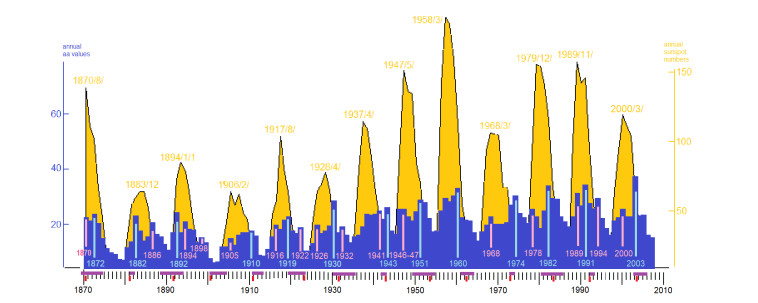
[11] | NOAA, Annual sunspots and aa index. Available from: https://www.ngdc.noaa.gov/stp/geomag/image/aassn07.jpg. |
[12] | AA index, graphs for 2000–2020. Available from: https://www.spaceweatherlive.com/community/topic/1553-ap-aa-indices-and-solar-minimum/, https://twitter.com/peikko763/status/1235142277842046976. |
1. | Agustín Moreno Cañadas, Adolfo Ballester-Bolinches, Isaías David Marín Gaviria, Solutions of the Yang–Baxter Equation Arising from Brauer Configuration Algebras, 2022, 11, 2079-3197, 2, 10.3390/computation11010002 | |
2. | Agustín Moreno Cañadas, Gabriel Bravo Rios, Robinson-Julian Serna, Snake Graphs Arising from Groves with an Application in Coding Theory, 2022, 10, 2079-3197, 124, 10.3390/computation10070124 | |
3. | Agustín Moreno Cañadas, Pedro Fernando Fernández Espinosa, Adolfo Ballester-Bolinches, Solutions of the Yang–Baxter Equation and Automaticity Related to Kronecker Modules, 2023, 11, 2079-3197, 43, 10.3390/computation11030043 |
Algorithm 1: Construction of a Brauer configuration algebra |
1. Input A reduced Brauer configuration Γ=(Γ0,Γ1,μ,O). |
2. Output The Brauer configuration algebra ΛΓ=FQΓ/IΓ |
3. Construct the quiver QΓ=((QΓ)0,(QΓ)1,s:(QΓ)1→(QΓ)0,t:(QΓ)1→(QΓ)0) |
(a) (QΓ)0=Γ1, |
(b) For each cover Ui<Ui+1∈Γ1 define an arrow a∈(QΓ)1, such that s(a)=Ui and t(a)=Ui+1, |
(c) Each relation Ui<Ui defines a loop in QΓ, |
(d) Each ordered set Sα defines a cycle Cα=Sα∪{Uim<Ui1} in QΓ called special cycle. Special cycles are obtained from successor sequences by defining a suitable circular relation, without loss of generality, we assume that a relation of the form Uim<Ui1 holds in special cycles. |
4. Define the path algebra FQΓ, |
5. Construct the admissible ideal IΓ, which is generated by the following relations: |
(a) If αi,αj∈U, U∈Γ1 and Cαi,Cαj are corresponding special cycles then Cμ(αi)αi−Cμ(αj)αj=0, |
(b) If Cαi is a special cycle associated to the vertex αi then Cμ(αi)a=0, if a is the first arrow of Cαi, |
(c) If α,α′∈Γ0, α≠α′, a,b∈(QΓ)1, a≠b, ab∉Cα for any α∈Γ0 then ab=0, if a∈Cα, b∈Cα′ and ab∈FQΓ, |
(d) If a is a loop associated to a vertex α with val(α)=1 and μ(α)>1 then aμ(α)+1=0. |
6. ΛΓ=FQΓ/IΓ is the Brauer configuration algebra. |
7. For the construction of a basis of ΛΓ follow the next steps: |
(a) For each U∈Γ1 choose a non-truncated vertex αU and exactly one special α-cycle CαU at U, |
(b) Define: |
A={¯p∣pisaproperprefixofsomeCμ(α)α},B={¯Cμ(α)αU∣U∈Γ1}. |
(c) A∪B is a F-basis of ΛΓ. |