Water resources management versus the world

John Greenway; John Greenway

doi:10.3934/geosci.2021035

AIMS Geosciences

2021, Volume 7, Issue 4: 589-604. doi: 10.3934/geosci.2021035

Previous Article Next Article

Research article

Water resources management versus the world

John Greenway ^,

School of Education, HASSE, University of New England, Armidale, NSW, Australia

Received: 06 September 2021 Accepted: 01 November 2021 Published: 03 November 2021

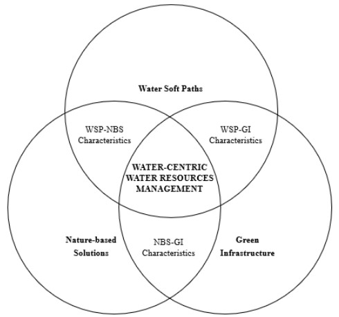
Effective water resources management and water availability are under threat from multiple sources, including population growth, continuing urbanisation, and climate change. In this context, current water resources management requires a conceptual rethink, which is lacking in the urban water resources management literature. This paper addresses this gap by rethinking urban water resources management from a water-centric perspective. The paper discusses a conceptual rethinking of water resources management towards a water-centric water resources management system underpinned through combining nature-based solutions (NBS), green infrastructure, and water soft path approaches. It is concluded that through adopting a blend of NBS, green infrastructure, and water soft paths, a water-centric water resources management approach focused on achieving sustainable water availability can be developed. It is further concluded that in transitioning to a water-centric focused water resources management approach, water needs to be acknowledged as a key stakeholder in relation to guiding a transition to an effective holistic catchment-wide water-centric water resources management system focused on achieving sustainable water availability.

Keywords:

Citation: John Greenway. Water resources management versus the world[J]. AIMS Geosciences, 2021, 7(4): 589-604. doi: 10.3934/geosci.2021035

Related Papers:

[1]	Ruifang Yang, Shilin Yang . Representations of a non-pointed Hopf algebra. AIMS Mathematics, 2021, 6(10): 10523-10539. doi: 10.3934/math.2021611
[2]	Fengxia Gao, Jialei Chen . Conjugacy classes of left ideals of Sweedler's four-dimensional algebra $H_{4}$ . AIMS Mathematics, 2022, 7(5): 7720-7727. doi: 10.3934/math.2022433
[3]	Haijun Cao, Fang Xiao . The category of affine algebraic regular monoids. AIMS Mathematics, 2022, 7(2): 2666-2679. doi: 10.3934/math.2022150
[4]	Yaguo Guo, Shilin Yang . Projective class rings of a kind of category of Yetter-Drinfeld modules. AIMS Mathematics, 2023, 8(5): 10997-11014. doi: 10.3934/math.2023557
[5]	Faiza Shujat, Faarie Alharbi, Abu Zaid Ansari . Weak $(p, q)$ -Jordan centralizer and derivation on rings and algebras. AIMS Mathematics, 2025, 10(4): 8322-8330. doi: 10.3934/math.2025383
[6]	Mingze Zhao, Huilan Li . A pair of dual Hopf algebras on permutations. AIMS Mathematics, 2021, 6(5): 5106-5123. doi: 10.3934/math.2021302
[7]	Panpan Jia, Jizhu Nan, Yongsheng Ma . Separating invariants for certain representations of the elementary Abelian $p$ -groups of rank two. AIMS Mathematics, 2024, 9(9): 25603-25618. doi: 10.3934/math.20241250
[8]	Zehra Velioǧlu, Mukaddes Balçik . On the Tame automorphisms of differential polynomial algebras. AIMS Mathematics, 2020, 5(4): 3547-3555. doi: 10.3934/math.2020230
[9]	Qining Li . Double Ore extensions of anti-angle type for Hopf algebras. AIMS Mathematics, 2022, 7(7): 12566-12586. doi: 10.3934/math.2022696
[10]	Simone Costa, Marco Pavone . Orthogonal and oriented Fano planes, triangular embeddings of $K_7,$ and geometrical representations of the Frobenius group $F_{21}$ . AIMS Mathematics, 2024, 9(12): 35274-35292. doi: 10.3934/math.20241676

Abstract

1. Motivations and outline

In [,Definition 11.2] and [,p. 134,Theorem A], the second kind Bell polynomials ${\rm{B}}_{n, k}$ for $n\ge k\ge0$ are defined by

$\begin{equation*} {\rm{B}}_{n,k}(x_1,x_2,\dotsc,x_{n-k+1}) = \sum\limits_{\ell\in\mathbb{N}_0^{n-k+1}}\frac{n!}{\prod_{i = 1}^{n-k+1}\ell_i!} \prod\limits_{i = 1}^{n-k+1}\biggl(\frac{x_i}{i!}\biggr)^{\ell_i}, \end{equation*}$

where $\mathbb{N}_0 = \{0\}\cup\mathbb{N}$ , the sum is taken over $\ell = (\ell_1, \ell_2, \dotsc, \ell_{n-k+1})$ with $\ell_i\in\mathbb{N}_0$ satisfying $\sum_{i = 1}^{n-k+1}\ell_i = k$ and $\sum_{i = 1}^{n-k+1}i\ell_i = n$ . This kind of polynomials are very important in combinatorics, analysis, and the like. See the review and survey article ^[53] and closely related references therein.

In [36,pp. 13–15], when studying Grothendieck's inequality and completely correlation-preserving functions, Oertel obtained the interesting identity

$\begin{equation*} \sum\limits_{k = 1}^{2n}(-1)^k\frac{(2n+k)!}{k!} {\rm{B}}_{2n,k}^{\circ}\biggl(0,\frac{1}{6},0,\frac{3}{40},0,\frac{5}{112},\dotsc, \frac{1+(-1)^{k+1}}{2}\frac{[(2n-k)!!]^2}{(2n-k+2)!}\biggr) = (-1)^n \end{equation*}$

for $n\in\mathbb{N}$ , where

$\begin{equation} {\rm{B}}_{n,k}^{\circ}(x_1,x_2,\dotsc,x_{n-k+1}) = \frac{k!}{n!}{\rm{B}}_{n,k}(1!x_1,2!x_2,\dotsc,(n-k+1)!x_{n-k+1}). \end{equation}$

(1.1)

In [36,p. 15], Oertel wrote that "However, already in this case we don't know a closed form expression for the numbers

$\begin{equation} {\rm{B}}_{2n,k}^{\circ}\biggl(0,\frac{1}{6},0,\frac{3}{40},0,\frac{5}{112},\dotsc, \frac{1+(-1)^{k+1}}{2}\frac{[(2n-k)!!]^2}{(2n-k+2)!}\biggr). \end{equation}$

(1.2)

An even stronger problem appears in the complex case, since already a closed-form formula for the coefficients of the Taylor series of the inverse of the Haagerup function is still unknown''.

By virtue of the relation (1.1), we see that, to find a closed-form formula for the sequence (1.2), it suffices to discover a closed-form formula for

$\begin{equation} {\rm{B}}_{2n,k}\biggl(0,\frac{1}{3},0,\frac{9}{5},0,\frac{225}{7},\dotsc, \frac{1+(-1)^{k+1}}{2}\frac{[(2n-k)!!]^2}{2n-k+2}\biggr). \end{equation}$

(1.3)

In this paper, one of our aims is to derive closed-form formulas for the sequence (1.3). The first main result can be stated as the following theorem.

Theorem 1.1. For $k, n\ge0$ , $m\in\mathbb{N}$ , and $x_{m}\in\mathbb{C}$ , we have

$\begin{equation} {\rm{B}}_{2n+1,k}\biggl(0,x_2,0,x_4,\dotsc,\frac{1+(-1)^{k}}{2}x_{2n-k+2}\biggr) = 0. \end{equation}$

(1.4)

For $k, n\in\mathbb{N}$ , we have

$\begin{align*} &\quad{\rm{B}}_{2n,2k-1}\biggl(0,\frac{1}{3},0,\frac{9}{5},0,\frac{225}{7},\dotsc, 0, \frac{[(2n-2k+1)!!]^2}{2n-2k+3}\biggr)\\ & = \frac{2^{2n}}{(2k-1)!}\Biggl[\sum\limits_{p = 1}^{k}(-4)^{p-1}\frac{\binom{2k-1}{2p-1}}{\binom{2n+2p-1}{2p-1}} \sum\limits_{q = 0}^{2p-2}T\biggl(n+p-1;q,2p-2;\frac{1}{2}\biggr)\\ &\quad-\sum\limits_{p = 1}^{k-1}(-1)^{p-1}\frac{\binom{2k-1}{2p}}{\binom{2n+2p}{2p}} \sum\limits_{q = 0}^{2p-2} T(n+p-1;q,2p-2;1)\Biggr] \end{align*}$

and

$\begin{align*} &\quad{\rm{B}}_{2n,2k}\biggl(0,\frac{1}{3},0,\frac{9}{5},0,\frac{225}{7},\dotsc,\frac{[(2n-2k-1)!!]^2}{2n-2k+1},0\biggr)\\ & = \frac{2^{2n}}{(2k)!}\Biggl[\sum\limits_{p = 1}^{k}(-1)^{p-1}\frac{\binom{2k}{2p}}{\binom{2n+2p}{2p}} \sum\limits_{q = 0}^{2p-2} T(n+p-1;q,2p-2;1)\\ &\quad-\sum\limits_{p = 1}^{k}(-4)^{p-1}\frac{\binom{2k}{2p-1}}{\binom{2n+2p-1}{2p-1}} \sum\limits_{q = 0}^{2p-2} T\biggl(n+p-1;q,2p-2;\frac{1}{2}\biggr)\Biggr], \end{align*}$

where $s(n, k)$ , which can be generated by

$\begin{equation} \langle x\rangle_n = \sum\limits_{m = 0}^{n}s(n,m)x^m, \end{equation}$

(1.5)

denote the first kind Stirling numbers and

$\begin{equation} T(r;q,j;\rho) = (-1)^q\Biggl[\sum\limits_{m = q}^{r}(-\rho)^{m}s(r,m)\binom{m}{q}\Biggr] \Biggl[\sum\limits_{m = j-q}^{r}(-\rho)^{m}s(r,m)\binom{m}{j-q}\Biggr]. \end{equation}$

(1.6)

In Section 2, for proving Theorem 1.1, we will establish two general expressions for power series expansions of $(\arcsin x)^{2\ell-1}$ and $(\arcsin x)^{2\ell}$ respectively.

In Section 3, with the aid of general expressions for power series expansions of the functions $(\arcsin x)^{2\ell-1}$ and $(\arcsin x)^{2\ell}$ established in Section 2, we will prove Theorem 1.1 in details.

In Section 4, basing on arguments in [,p. 308] and [,Section 2.4] and utilizing general expressions for power series expansions of $(\arcsin x)^{2\ell-1}$ and $(\arcsin x)^{2\ell}$ established in Section 2, we will derive series representations of generalized logsine functions which were originally introduced in ^[34] and have been investigating actively, deeply, and systematically by mathematicians ^{[9,10,14,15,16,17,29,30,31,37,38,57]} and physicists ^[3,19,20,28].

Finally, in Section 5, we will list several remarks on our main results and related stuffs.

2. Power series expansions for the powers of the arcsine function

To prove Theorem 1.1, we need to establish the following general expressions of the power series expansions of $(\arcsin x)^\ell$ for $\ell\in\mathbb{N}$ .

Theorem 2.1. For $\ell\in\mathbb{N}$ and $|x| < 1$ , the functions $(\arcsin x)^\ell$ can be expanded into power series

$\begin{equation} (\arcsin x)^{2\ell-1} = (-4)^{\ell-1}\sum\limits_{n = 0}^{\infty}\frac{4^{n}}{(2n)!}\Biggl[\sum\limits_{q = 0}^{2\ell-2}T\biggl(n+\ell-1;q,2\ell-2;\frac12\biggr)\Biggr] \frac{x^{2n+2\ell-1}}{\binom{2n+2\ell-1}{2\ell-1}} \end{equation}$

(2.1)

$\begin{equation} (\arcsin x)^{2\ell} = (-1)^{\ell-1}\sum\limits_{n = 0}^{\infty}\frac{4^{n}}{(2n)!} \Biggl[\sum\limits_{q = 0}^{2\ell-2}T(n+\ell-1;q,2\ell-2;1)\Biggr] \frac{x^{2n+2\ell}}{\binom{2n+2\ell}{2\ell}}, \end{equation}$

(2.2)

where $s(n, k)$ denotes the first kind Stirling numbers generated in (1.5) and $T(r; q, j;\rho)$ is defined by (1.6).

Proof. In [4,pp. 262–263,Proposition 15], [,p. 3], [,p. 308], and [,pp. 49–50], it was stated that the generating expression for the series expansion of $(\arcsin x)^n$ with $n\in\mathbb{N}$ is

$\begin{equation*} \exp(t\arcsin x) = \sum\limits_{\ell = 0}^{\infty}\frac{b_\ell(t)x^\ell}{\ell!}, \end{equation*}$

where $b_0(t) = 1$ , $b_1(t) = t$ , and

$\begin{equation*} b_{2\ell}(t) = \prod\limits_{k = 0}^{\ell-1}\bigl[t^2+(2k)^2\bigr], \quad b_{2\ell+1}(t) = t\prod\limits_{k = 1}^{\ell}\bigl[t^2+(2k-1)^2\bigr] \end{equation*}$

for $\ell\in\mathbb{N}$ . This means that, when writing

$\begin{equation*} b_\ell(t) = \sum\limits_{k = 0}^{\ell}\beta_{\ell,k}t^{k},\quad \ell\ge0, \end{equation*}$

where $\beta_{0, 0} = 1$ , $\beta_{2\ell, 0} = 0$ , $\beta_{2\ell, 2k+1} = 0$ , and $\beta_{2\ell-1, 2k} = 0$ for $k\ge0$ and $\ell\ge1$ , we have

$\begin{equation*} \sum\limits_{\ell = 0}^{\infty}(\arcsin x)^\ell\frac{t^\ell}{\ell!} = \sum\limits_{\ell = 0}^{\infty}\frac{x^\ell}{\ell!}\sum\limits_{k = 0}^{\ell}\beta_{\ell,k}t^{k} = \sum\limits_{k = 0}^{\infty}\sum\limits_{\ell = k}^{\infty}\frac{x^\ell}{\ell!}\beta_{\ell,k}t^{k} = \sum\limits_{\ell = 0}^{\infty}\Biggl[\sum\limits_{m = \ell}^{\infty}\beta_{m,\ell}\frac{x^m}{m!}\Biggr]t^{\ell}. \end{equation*}$

Equating coefficients of $t^\ell$ gives

$\begin{equation} (\arcsin x)^\ell = \ell!\sum\limits_{m = \ell}^{\infty}\beta_{m,\ell}\frac{x^m}{m!} = \ell!\sum\limits_{n = 0}^{\infty}\beta_{n+\ell,\ell}\frac{x^{n+\ell}}{(n+\ell)!}, \quad \ell\in\mathbb{N}. \end{equation}$

(2.3)

It is not difficult to see that

$\begin{equation*} b_{2\ell}(t) = 4^{\ell-1} t^2\biggl(1-\frac{i t}{2}\biggr)_{\ell-1} \biggl(1+\frac{i t}{2}\biggr)_{\ell-1} \quad{\rm{and}}\quad b_{2\ell+1}(t) = 4^\ell t\biggl(\frac{1}{2}-\frac{i t}{2}\biggr)_\ell \biggl(\frac{1}{2}+\frac{i t}{2}\biggr)_\ell, \end{equation*}$

where $i = \sqrt{-1}\,$ is the imaginary unit and

$\begin{equation*} (z)_n = \prod\limits_{\ell = 0}^{n-1}(z+\ell) = \begin{cases} z(z+1)\dotsm(z+n-1), & n\ge1\\ 1, & n = 0 \end{cases} \end{equation*}$

is called the rising factorial of $z\in\mathbb{C}$ , while

$\begin{equation} \langle z\rangle_n = \prod\limits_{\ell = 0}^{n-1}(z-\ell) = \begin{cases} z(z-1)\dotsm(z-n+1), & n\ge1\\ 1,& n = 0 \end{cases} \end{equation}$

(2.4)

is called the falling factorial of $z\in\mathbb{C}$ . Making use of the relation

$\begin{equation*} (-z)_n = (-1)^n\langle z\rangle_n\quad {\rm{or}}\quad \langle-z\rangle_n = (-1)^n(z)_n \end{equation*}$

in [52,p. 167], we acquire

$\begin{equation*} b_{2\ell}(t) = 4^{\ell-1} t^2\biggl\langle\frac{i t}{2}-1\biggr\rangle_{\ell-1} \biggl\langle-\frac{i t}{2}-1\biggr\rangle_{\ell-1} \quad{\rm{and}}\quad b_{2\ell+1}(t) = 4^\ell t\biggl\langle\frac{i t}{2}-\frac{1}{2}\biggr\rangle_\ell \biggl\langle-\frac{i t}{2}-\frac{1}{2}\biggr\rangle_\ell. \end{equation*}$

Utilizing the relation (1.5) in [59,p. 19,(1.26)], we obtain

$\begin{align*} b_{2\ell}(t)& = 4^{\ell-1} t^2\sum\limits_{m = 0}^{\ell-1}\frac{s(\ell-1,m)}{2^m}(it-2)^{m} \sum\limits_{m = 0}^{\ell-1}(-1)^{m}\frac{s(\ell-1,m)}{2^{m}}(it+2)^{m}\\ & = 4^{\ell-1} t^2\sum\limits_{m = 0}^{\ell-1}\frac{s(\ell-1,m)}{2^{m}} \sum\limits_{k = 0}^{m}\binom{m}{k}i^kt^k(-2)^{m-k} \sum\limits_{m = 0}^{\ell-1}(-1)^{m}\frac{s(\ell-1,m)}{2^{m}} \sum\limits_{k = 0}^{m}\binom{m}{k}i^kt^k2^{m-k}\\ & = 4^{\ell-1} t^2\sum\limits_{m = 0}^{\ell-1}(-1)^{m}s(\ell-1,m) \sum\limits_{k = 0}^{m}\frac{(-1)^{k}}{2^{k}}\binom{m}{k}i^kt^k \sum\limits_{m = 0}^{\ell-1}(-1)^{m}s(\ell-1,m)\sum\limits_{k = 0}^{m} \frac1{2^{k}}\binom{m}{k}i^kt^k\\ & = 4^{\ell-1} t^2\sum\limits_{k = 0}^{\ell-1}\Biggl[\sum\limits_{m = k}^{\ell-1}(-1)^{m+k}\frac{s(\ell-1,m)}{2^{k}}\binom{m}{k}\Biggr]i^kt^k \sum\limits_{k = 0}^{\ell-1}\Biggl[\sum\limits_{m = k}^{\ell-1}(-1)^{m} \frac{s(\ell-1,m)}{2^{k}}\binom{m}{k}\Biggr]i^kt^k\\ & = 4^{\ell-1} t^2\sum\limits_{k = 0}^{2(\ell-1)}\sum\limits_{q = 0}^{k} \Biggl[\sum\limits_{m = q}^{\ell-1}(-1)^{m+q}\frac{s(\ell-1,m)}{2^{q}}\binom{m}{q} \sum\limits_{m = k-q}^{\ell-1}(-1)^{m}\frac{s(\ell-1,m)}{2^{k-q}}\binom{m}{k-q}\Biggr]i^kt^k\\ & = 4^{\ell-1} t^2\sum\limits_{k = 0}^{2(\ell-1)}\frac{1}{2^k} \sum\limits_{q = 0}^{k}\Biggl[\sum\limits_{m = q}^{\ell-1}(-1)^{m+q}s(\ell-1,m)\binom{m}{q} \sum\limits_{m = k-q}^{\ell-1}(-1)^{m}s(\ell-1,m)\binom{m}{k-q}\Biggr]i^kt^k\\ & = 4^{\ell-1}\sum\limits_{k = 0}^{2(\ell-1)}\frac{i^k}{2^k} \Biggl[\sum\limits_{q = 0}^{k} \Biggl(\sum\limits_{m = q}^{\ell-1}(-1)^{m}s(\ell-1,m)\binom{m}{q}\Biggr) \sum\limits_{m = k-q}^{\ell-1}(-1)^{m}s(\ell-1,m)\binom{m}{k-q}\Biggr]t^{k+2}\\ & = 4^{\ell-1}\sum\limits_{k = 0}^{2(\ell-1)}\frac{i^k}{2^k} \Biggl[\sum\limits_{q = 0}^{k}T(\ell-1;q,k;1)\Biggr]t^{k+2} \end{align*}$

and

$\begin{align*} b_{2\ell+1}(t)& = 4^\ell t \sum\limits_{m = 0}^{\ell}\frac{s(\ell,m)}{2^m}(it-1)^m \sum\limits_{m = 0}^{\ell}(-1)^m\frac{s(\ell,m)}{2^m}(it+1)^m\\ & = 4^\ell t \sum\limits_{m = 0}^{\ell}\frac{s(\ell,m)}{2^m}\sum\limits_{k = 0}^{m}(-1)^{m-k}\binom{m}{k}i^kt^k \sum\limits_{m = 0}^{\ell}(-1)^m\frac{s(\ell,m)}{2^m}\sum\limits_{k = 0}^{m}\binom{m}{k}i^kt^k\\ & = 4^\ell t \sum\limits_{k = 0}^{\ell}\Biggl[\sum\limits_{m = k}^{\ell}(-1)^{m}\frac{s(\ell,m)}{2^m}\binom{m}{k}\Biggr](-i)^kt^k \sum\limits_{k = 0}^{\ell}\Biggl[\sum\limits_{m = k}^{\ell}(-1)^m\frac{s(\ell,m)}{2^m}\binom{m}{k}\Biggr]i^kt^k\\ & = 4^\ell\sum\limits_{k = 0}^{2\ell}i^k\Biggl[\sum\limits_{q = 0}^{k}(-1)^q\Biggl(\sum\limits_{m = q}^{\ell}(-1)^m\frac{s(\ell,m)}{2^m}\binom{m}{q}\Biggr) \sum\limits_{m = k-q}^{\ell}(-1)^m\frac{s(\ell,m)}{2^m}\binom{m}{k-q}\Biggr]t^{k+1}\\ & = 4^\ell\sum\limits_{k = 0}^{2\ell}i^k\Biggl[\sum\limits_{q = 0}^{k}T\biggl(\ell;q,k;\frac{1}{2}\biggr)\Biggr]t^{k+1}. \end{align*}$

This means that

$\begin{equation*} \sum\limits_{k = 0}^{2\ell}\beta_{2\ell,k}t^{k} = \sum\limits_{k = -2}^{2(\ell-1)}\beta_{2\ell,k+2}t^{k+2} = \sum\limits_{k = 0}^{2(\ell-1)}\beta_{2\ell,k+2}t^{k+2} = 4^{\ell-1}\sum\limits_{k = 0}^{2(\ell-1)}\frac{i^k}{2^k} \Biggl[\sum\limits_{q = 0}^{k}T(\ell-1;q,k;1)\Biggr]t^{k+2} \end{equation*}$

and

$\begin{equation*} \sum\limits_{k = 0}^{2\ell+1}\beta_{2\ell+1,k}t^{k} = \sum\limits_{k = -1}^{2\ell}\beta_{2\ell+1,k+1}t^{k+1} = \sum\limits_{k = 0}^{2\ell}\beta_{2\ell+1,k+1}t^{k+1} = 4^\ell\sum\limits_{k = 0}^{2\ell}i^k\Biggl[\sum\limits_{q = 0}^{k}T\biggl(\ell;q,k;\frac{1}{2}\biggr)\Biggr]t^{k+1}. \end{equation*}$

Further equating coefficients of $t^{k+2}$ and $t^{k+1}$ respectively arrives at

$\begin{equation*} \beta_{2\ell,k+2} = 4^{\ell-1}\frac{i^k}{2^k} \sum\limits_{q = 0}^{k}T(\ell-1;q,k;1) \quad{\rm{and}}\quad \beta_{2\ell+1,k+1} = 4^\ell i^k\sum\limits_{q = 0}^{k}T\biggl(\ell;q,k;\frac{1}{2}\biggr) \end{equation*}$

for $k\ge0$ .

Replacing $\ell$ by $2\ell-1$ for $\ell\in\mathbb{N}$ in (2.3) leads to

$\begin{align*} (\arcsin x)^{2\ell-1}& = (2\ell-1)!\sum\limits_{n = 0}^{\infty}\beta_{n+2\ell-1,2\ell-1}\frac{x^{n+2\ell-1}}{(n+2\ell-1)!}\\ & = (2\ell-1)!\sum\limits_{n = 0}^{\infty}\beta_{2n+2\ell-1,2\ell-1}\frac{x^{2n+2\ell-1}}{(2n+2\ell-1)!}\\ & = (2\ell-1)!\sum\limits_{n = 0}^{\infty}\Biggl[4^{n+\ell-1}i^{2(\ell-1)} \sum\limits_{q = 0}^{2(\ell-1)}T\biggl(n+\ell-1;q,2\ell-2;\frac{1}{2}\biggr)\Biggr] \frac{x^{2n+2\ell-1}}{(2n+2\ell-1)!}\\ & = (-1)^{\ell-1}4^{\ell-1}(2\ell-1)!\sum\limits_{n = 0}^{\infty}\Biggl[4^{n}\sum\limits_{q = 0}^{2(\ell-1)} T\biggl(n+\ell-1;q,2\ell-2;\frac{1}{2}\biggr)\Biggr] \frac{x^{2n+2\ell-1}}{(2n+2\ell-1)!}\\ & = (-4)^{\ell-1}\sum\limits_{n = 0}^{\infty}\frac{4^{n}}{(2n)!}\Biggl[\sum\limits_{q = 0}^{2\ell-2}T\biggl(n+\ell-1;q,2\ell-2;\frac12\biggr)\Biggr] \frac{x^{2n+2\ell-1}}{\binom{2n+2\ell-1}{2\ell-1}}. \end{align*}$

Replacing $\ell$ by $2\ell$ for $\ell\in\mathbb{N}$ in (2.3) leads to

$\begin{align*} (\arcsin x)^{2\ell}& = (2\ell)!\sum\limits_{n = 0}^{\infty}\beta_{n+2\ell,2\ell}\frac{x^{n+2\ell}}{(n+2\ell)!}\\ & = (2\ell)!\sum\limits_{n = 0}^{\infty}\beta_{2n+2\ell,2\ell}\frac{x^{2n+2\ell}}{(2n+2\ell)!}\\ & = (-1)^{\ell-1}(2\ell)!\sum\limits_{n = 0}^{\infty}\Biggl[4^{n} \sum\limits_{q = 0}^{2(\ell-1)} T(n+\ell-1;q,2\ell-2;1)\Biggr]\frac{x^{2n+2\ell}}{(2n+2\ell)!}\\ & = (-1)^{\ell-1}\sum\limits_{n = 0}^{\infty}\frac{4^{n}}{(2n)!} \Biggl[\sum\limits_{q = 0}^{2\ell-2}T(n+\ell-1;q,2\ell-2;1)\Biggr] \frac{x^{2n+2\ell}}{\binom{2n+2\ell}{2\ell}}. \end{align*}$

The proof of Theorem 2.1 is complete.

3. Proof of Theorem 1.1

We now start out to prove Theorem 1.1.

In the last line of [18,p. 133], there exists the formula

$\begin{equation} \frac1{k!}\Biggl(\sum\limits_{m = 1}^\infty x_m\frac{t^m}{m!}\Biggr)^k = \sum\limits_{n = k}^\infty {\rm{B}}_{n,k}(x_1,x_2,\dotsc,x_{n-k+1})\frac{t^n}{n!} \end{equation}$

(3.1)

for $k\ge0$ . When taking $x_{2m-1} = 0$ for $m\in\mathbb{N}$ , the left hand side of the formula (3.1) is even in $t\in(-\infty, \infty)$ for all $k\ge0$ . Therefore, the formula (1.4) is valid.

Ones know that the power series expansion

$\begin{equation} \arcsin t = \sum\limits_{\ell = 0}^{\infty}\frac{[(2\ell-1)!!]^2}{(2\ell+1)!}t^{2\ell+1},\quad |t| < 1 \end{equation}$

(3.2)

is valid, where $(-1)!! = 1$ . This implies that

$\begin{gather*} {\rm{B}}_{2n,k}\biggl(0,\frac{1}{3},0,\frac{9}{5},0,\frac{225}{7},\dotsc, \frac{1+(-1)^{k+1}}{2}\frac{[(2n-k)!!]^2}{2n-k+2}\biggr)\\ = {\rm{B}}_{2n,k}\biggl(\frac{(\arcsin t)''|_{t = 0}}{2}, \frac{(\arcsin t)'''|_{t = 0}}{3}, \frac{(\arcsin t)^{(4)}|_{t = 0}}{4},\dotsc, \frac{(\arcsin t)^{(2n-k+2)}|_{t = 0}}{2n-k+2}\biggr). \end{gather*}$

Employing the formula

$\begin{equation*} {\rm{B}}_{n,k}\biggl(\frac{x_2}{2},\frac{x_3}{3},\dotsc,\frac{x_{n-k+2}}{n-k+2}\biggr) = \frac{n!}{(n+k)!}{\rm{B}}_{n+k,k}(0,x_2,x_3,\dotsc,x_{n+1}) \end{equation*}$

in [18,p. 136], we derive

$\begin{gather*} {\rm{B}}_{2n,k}\biggl(0,\frac{1}{3},0,\frac{9}{5},0,\frac{225}{7},\dotsc, \frac{1+(-1)^{k+1}}{2}\frac{[(2n-k)!!]^2}{2n-k+2}\biggr)\\ = \frac{(2n)!}{(2n+k)!}{\rm{B}}_{2n+k,k}\bigl(0,(\arcsin t)''|_{t = 0},(\arcsin t)'''|_{t = 0},\dotsc,(\arcsin t)^{(2n+1)}|_{t = 0}\bigr). \end{gather*}$

Making use of the formula (3.1) yields

$\begin{align*} \sum\limits_{n = 0}^\infty {\rm{B}}_{n+k,k}(x_1,x_2,\dotsc,x_{n+1})\frac{k!n!}{(n+k)!}\frac{t^{n+k}}{n!} & = \Biggl(\sum\limits_{m = 1}^\infty x_m\frac{t^m}{m!}\Biggr)^k,\\ \sum\limits_{n = 0}^\infty \frac{{\rm{B}}_{n+k,k}(x_1,x_2,\dotsc,x_{n+1})}{\binom{n+k}{k}}\frac{t^{n+k}}{n!} & = \Biggl(\sum\limits_{m = 1}^\infty x_m\frac{t^m}{m!}\Biggr)^k,\\ {\rm{B}}_{n+k,k}(x_1,x_2,\dotsc,x_{n+1}) & = \binom{n+k}{k}\lim\limits_{t\to0}\frac{{\rm{d}}^n}{{\rm{d}} t^n}\Biggl[\sum\limits_{m = 0}^\infty x_{m+1}\frac{t^{m}}{(m+1)!}\Biggr]^k,\\ {\rm{B}}_{2n+k,k}(x_1,x_2,\dotsc,x_{2n+1}) & = \binom{2n+k}{k}\lim\limits_{t\to0}\frac{{\rm{d}}^{2n}}{{\rm{d}} t^{2n}}\Biggl[\sum\limits_{m = 0}^\infty x_{m+1}\frac{t^{m}}{(m+1)!}\Biggr]^k. \end{align*}$

Setting $x_1 = 0$ and $x_m = (\arcsin t)^{(m)}|_{t = 0}$ for $m\ge2$ gives

$\begin{align*} \frac{{\rm{d}}^{2n}}{{\rm{d}} t^{2n}}\Biggl[\sum\limits_{m = 0}^\infty x_{m+1}\frac{t^{m}}{(m+1)!}\Biggr]^k & = \frac{{\rm{d}}^{2n}}{{\rm{d}} t^{2n}}\Biggl[\frac{1}{t} \sum\limits_{m = 2}^\infty (\arcsin t)^{(m)}|_{t = 0} \frac{t^m}{m!}\Biggr]^k\\ & = \frac{{\rm{d}}^{2n}}{{\rm{d}} t^{2n}}\biggl(\frac{\arcsin t-t}{t}\biggr)^k\\ & = \frac{{\rm{d}}^{2n}}{{\rm{d}} t^{2n}}\sum\limits_{p = 0}^{k}(-1)^{k-p}\binom{k}{p}\biggl(\frac{\arcsin t}{t}\biggr)^p\\ & = \sum\limits_{p = 1}^{k}(-1)^{k-p}\binom{k}{p}\frac{{\rm{d}}^{2n}}{{\rm{d}} t^{2n}}\biggl(\frac{\arcsin t}{t}\biggr)^p. \end{align*}$

Accordingly, we obtain

$\begin{gather*} \lim\limits_{t\to0}\frac{{\rm{d}}^{2n}}{{\rm{d}} t^{2n}}\Biggl[\frac{1}{t}\sum\limits_{m = 2}^\infty (\arcsin t)^{(m)}|_{t = 0}\frac{t^m}{m!}\Biggr]^{2k-1} = \sum\limits_{p = 1}^{2k-1}(-1)^{2k-p-1}\binom{2k-1}{p}\lim\limits_{t\to0}\frac{{\rm{d}}^{2n}}{{\rm{d}} t^{2n}}\biggl(\frac{\arcsin t}{t}\biggr)^p\\ = \sum\limits_{p = 1}^{k}\binom{2k-1}{2p-1}\lim\limits_{t\to0}\frac{{\rm{d}}^{2n}}{{\rm{d}} t^{2n}}\biggl(\frac{\arcsin t}{t}\biggr)^{2p-1} -\sum\limits_{p = 1}^{k-1}\binom{2k-1}{2p}\lim\limits_{t\to0}\frac{{\rm{d}}^{2n}}{{\rm{d}} t^{2n}}\biggl(\frac{\arcsin t}{t}\biggr)^{2p} \end{gather*}$

and

$\begin{gather*} \lim\limits_{t\to0}\frac{{\rm{d}}^{2n}}{{\rm{d}} t^{2n}}\Biggl[\frac{1}{t}\sum\limits_{m = 2}^\infty (\arcsin t)^{(m)}|_{t = 0}\frac{t^m}{m!}\Biggr]^{2k} = \sum\limits_{p = 1}^{2k}(-1)^{2k-p}\binom{2k}{p}\lim\limits_{t\to0}\frac{{\rm{d}}^{2n}}{{\rm{d}} t^{2n}}\biggl(\frac{\arcsin t}{t}\biggr)^p\\ = \sum\limits_{p = 1}^{k}\binom{2k}{2p}\lim\limits_{t\to0}\frac{{\rm{d}}^{2n}}{{\rm{d}} t^{2n}}\biggl(\frac{\arcsin t}{t}\biggr)^{2p} -\sum\limits_{p = 1}^{k}\binom{2k}{2p-1}\lim\limits_{t\to0}\frac{{\rm{d}}^{2n}}{{\rm{d}} t^{2n}}\biggl(\frac{\arcsin t}{t}\biggr)^{2p-1}. \end{gather*}$

From the power series expansions (2.1) and (2.2) in Theorem 2.1, it follows that

$\begin{align*} \lim\limits_{t\to0}\frac{{\rm{d}}^{2n}}{{\rm{d}} t^{2n}}\biggl(\frac{\arcsin t}{t}\biggr)^{2p-1} & = (-1)^{p-1}4^{p-1}(2p-1)!\\ &\quad\times\lim\limits_{t\to0}\frac{{\rm{d}}^{2n}}{{\rm{d}} t^{2n}}\sum\limits_{j = 0}^{\infty}\Biggl[4^{j}\sum\limits_{q = 0}^{2p-2} T\biggl(j+p-1;q,2p-2;\frac12\biggr)\Biggr] \frac{t^{2j}}{(2j+2p-1)!}\\ & = (-1)^{p-1}\frac{4^{n+p-1}}{\binom{2n+2p-1}{2n}} \sum\limits_{q = 0}^{2p-2}T\biggl(n+p-1;q,2p-2;\frac12\biggr) \end{align*}$

and

$\begin{align*} \lim\limits_{t\to0}\frac{{\rm{d}}^{2n}}{{\rm{d}} t^{2n}}\biggl(\frac{\arcsin t}{t}\biggr)^{2p} & = (-1)^{p-1}(2p)!\lim\limits_{t\to0}\frac{{\rm{d}}^{2n}}{{\rm{d}} t^{2n}}\sum\limits_{j = 0}^{\infty}\Biggl[4^{j} \sum\limits_{q = 0}^{2p-2} T(j+p-1;q,2p-2;1)\Biggr]\frac{t^{2j}}{(2j+2p)!}\\ & = (-1)^{p-1}\frac{4^{n}}{\binom{2n+2p}{2n}} \sum\limits_{q = 0}^{2p-2} T(n+p-1;q,2p-2;1). \end{align*}$

Therefore, we arrive at

$\begin{align*} \lim\limits_{t\to0}\frac{{\rm{d}}^{2n}}{{\rm{d}} t^{2n}}\Biggl[\frac{1}{t}\sum\limits_{m = 2}^\infty (\arcsin t)^{(m)}|_{t = 0}\frac{t^m}{m!}\Biggr]^{2k-1} & = 4^n\sum\limits_{p = 1}^{k}(-4)^{p-1}\frac{\binom{2k-1}{2p-1}}{\binom{2n+2p-1}{2p-1}}\sum\limits_{q = 0}^{2p-2}T\biggl(n+p-1;q,2p-2;\frac12\biggr)\\ &\quad-4^{n}\sum\limits_{p = 1}^{k-1}(-1)^{p-1}\frac{\binom{2k-1}{2p}}{\binom{2n+2p}{2p}} \sum\limits_{q = 0}^{2p-2} T(n+p-1;q,2p-2;1) \end{align*}$

and

$\begin{align*} \lim\limits_{t\to0}\frac{{\rm{d}}^{2n}}{{\rm{d}} t^{2n}}\Biggl[\frac{1}{t}\sum\limits_{m = 2}^\infty (\arcsin t)^{(m)}|_{t = 0}\frac{t^m}{m!}\Biggr]^{2k} & = 4^{n}\sum\limits_{p = 1}^{k}(-1)^{p-1}\frac{\binom{2k}{2p}}{\binom{2n+2p}{2p}} \sum\limits_{q = 0}^{2p-2} T(n+p-1;q,2p-2;1)\\ &\quad-4^{n}\sum\limits_{p = 1}^{k}(-4)^{p-1}\frac{\binom{2k}{2p-1}}{\binom{2n+2p-1}{2p-1}} \sum\limits_{q = 0}^{2p-2}T\biggl(n+p-1;q,2p-2;\frac12\biggr). \end{align*}$

Consequently, we acquire

$\begin{align*} &\quad{\rm{B}}_{2n,2k-1}\biggl(0,\frac{1}{3},0,\frac{9}{5},0,\frac{225}{7},\dotsc, 0, \frac{[(2n-2k+1)!!]^2}{2n-2k+3}\biggr)\\ & = \frac{(2n)!}{(2n+2k-1)!}{\rm{B}}_{2n+2k-1,2k-1}\bigl(0,(\arcsin t)''|_{t = 0},(\arcsin t)'''|_{t = 0},\dotsc,(\arcsin t)^{(2n+1)}|_{t = 0}\bigr)\\ & = \frac{(2n)!}{(2n+2k-1)!}\binom{2n+2k-1}{2k-1} \lim\limits_{t\to0}\frac{{\rm{d}}^{2n}}{{\rm{d}} t^{2n}}\Biggl(\frac{1}{t}\sum\limits_{m = 2}^\infty (\arcsin t)^{(m)}|_{t = 0}\frac{t^m}{m!}\Biggr)^{2k-1}\\ & = \frac{1}{(2k-1)!}\Biggl[4^n\sum\limits_{p = 1}^{k}(-4)^{p-1}\frac{\binom{2k-1}{2p-1}}{\binom{2n+2p-1}{2p-1}} \sum\limits_{q = 0}^{2p-2}T\biggl(n+p-1;q,2p-2;\frac12\biggr)\\ &\quad-4^{n}\sum\limits_{p = 0}^{k-1}(-1)^{p-1}\frac{\binom{2k-1}{2p}}{\binom{2n+2p}{2p}} \sum\limits_{q = 0}^{2p-2} T(n+p-1;q,2p-2;1)\Biggr] \end{align*}$

and

$\begin{align*} &\quad{\rm{B}}_{2n,2k}\biggl(0,\frac{1}{3},0,\frac{9}{5},0,\frac{225}{7},\dotsc,\frac{[(2n-2k-1)!!]^2}{2n-2k+1},0\biggr)\\ & = \frac{(2n)!}{(2n+2k)!}{\rm{B}}_{2n+2k,2k}\bigl(0,(\arcsin t)''|_{t = 0},(\arcsin t)'''|_{t = 0},\dotsc,(\arcsin t)^{(2n+1)}|_{t = 0}\bigr)\\ & = \frac{(2n)!}{(2n+2k)!}\binom{2n+2k}{2k}\lim\limits_{t\to0}\frac{{\rm{d}}^{2n}}{{\rm{d}} t^{2n}}\Biggl(\frac{1}{t}\sum\limits_{m = 2}^\infty (\arcsin t)^{(m)}|_{t = 0}\frac{t^m}{m!}\Biggr)^{2k}\\ & = \frac{1}{(2k)!}\Biggl[4^{n}\sum\limits_{p = 1}^{k}(-1)^{p-1}\frac{\binom{2k}{2p}}{\binom{2n+2p}{2p}} \sum\limits_{q = 0}^{2p-2} T(n+p-1;q,2p-2;1)\\ &\quad-4^{n}\sum\limits_{p = 1}^{k}(-4)^{p-1}\frac{\binom{2k}{2p-1}}{\binom{2n+2p-1}{2p-1}} \sum\limits_{q = 0}^{2p-2} T\biggl(n+p-1;q,2p-2;\frac12\biggr)\Biggr]. \end{align*}$

The proof of Theorem 1.1 is complete.

4. Series representation of generalized logsine functions

The logsine function

$\begin{equation*} {\rm{Ls}}_j(\theta) = -\int_{0}^{\theta}\biggl(\ln\biggl|2\sin\frac{x}{2}\biggr|\biggr)^{j-1}{\rm{d}} x \end{equation*}$

and generalized logsine function

$\begin{equation*} {\rm{Ls}}_j^{(\ell)}(\theta) = -\int_{0}^{\theta}x^\ell\biggl(\ln\biggl|2\sin\frac{x}{2}\biggr|\biggr)^{j-\ell-1}{\rm{d}} x \end{equation*}$

were introduced originally in [,pp. 191–192], where $\ell, j$ are integers, $j\ge\ell+1\ge1$ , and $\theta$ is an arbitrary real number. There have been many papers such as ^{[3,9,10,14,15,16,17,19,20,28,29,30,31,37,38,57]} devoted to investigation and applications of the (generalized) logsine functions in mathematics, physics, engineering, and other mathematical sciences.

Theorem 4.1. Let $\langle z\rangle_n$ for $z\in\mathbb{C}$ and $n\in\{0\}\cup\mathbb{N}$ denote the falling factorial defined by (2.4) and let $T(r; q, j;\rho)$ be defined by (1.6). In the region $0 < \theta\le\pi$ and for $j, \ell\in\mathbb{N}$ , generalized logsine functions ${\rm{Ls}}_j^{(\ell)}(\theta)$ have the following series representations:

1. for $j\ge2\ell+1\ge3$ ,

$\begin{equation} \begin{aligned} {\rm{Ls}}_j^{(2\ell-1)}(\theta)& = -\frac{\theta^{2\ell}}{2\ell}\biggl[\ln\biggl(2\sin\frac{\theta}{2}\biggr)\biggr]^{j-2\ell} -(-1)^{\ell}(j-2\ell)(2\ell-1)!(\ln2)^{j-1}\biggl(\frac{2\sin\frac{\theta}{2}}{\ln2}\biggr)^{2\ell}\\ &\quad\times \sum\limits_{n = 0}^{\infty}\frac{\bigl(2\sin\frac{\theta}{2}\bigr)^{2n}}{(2n+2\ell)!} \Biggl[\sum\limits_{q = 0}^{2\ell-2} T(n+\ell-1;q,2\ell-2;1)\Biggr]\\ &\quad\times\Biggl[\sum\limits_{\alpha = 0}^{j-2\ell-1}\biggl(\frac{\ln\sin\frac{\theta}{2}}{\ln2}\biggr)^{\alpha} \binom{j-2\ell-1}{\alpha} \sum\limits_{k = 0}^{\alpha}\frac{(-1)^k\langle\alpha\rangle_{k}} {(2n+2\ell)^{k+1}\bigl(\ln\sin\frac{\theta}{2}\bigr)^{k}}\Biggr]; \end{aligned} \end{equation}$

(4.1)

2. for $j\ge2\ell+2\ge4$ ,

$\begin{equation} \begin{aligned} {\rm{Ls}}_j^{(2\ell)}(\theta)& = -\frac{\theta^{2\ell+1}}{2\ell+1}\biggl[\ln\biggl(2\sin\frac{\theta}{2}\biggr)\biggr]^{j-2\ell-1} +(-1)^{\ell}\frac{(j-2\ell-1)(2\ell)!(\ln2)^{j-1}}{2}\biggl(\frac{4\sin\frac{\theta}{2}}{\ln2}\biggr)^{2\ell+1}\\ &\quad\times\sum\limits_{n = 0}^{\infty}\Biggl[\frac{\bigl(2\sin\frac{\theta}{2}\bigr)^{2n}}{(2n+2\ell+1)!} \sum\limits_{q = 0}^{2\ell}T\biggl(n+\ell;q,2\ell;\frac12\biggr)\Biggr]\\ &\quad\times\Biggl[\sum\limits_{\alpha = 0}^{j-2\ell-2}\binom{j-2\ell-2}{\alpha}\biggl(\frac{\ln\sin\frac{\theta}{2}}{\ln2}\biggr)^\alpha \sum\limits_{k = 0}^{\alpha}\frac{(-1)^k\langle\alpha\rangle_{k}}{(2n+2\ell+1)^{k+1}\bigl(\ln\sin\frac{\theta}{2}\bigr)^{k}}\Biggr]; \end{aligned} \end{equation}$

(4.2)

3. for $j\ge2\ell-1\ge1$ ,

$\begin{equation} \begin{aligned} {\rm{Ls}}_j^{(2\ell-2)}(\theta)& = (-1)^{\ell}2^{4\ell-3}(2\ell-2)!(\ln2)^{j}\biggl(\frac{\sin\frac{\theta}{2}}{\ln2}\biggr)^{2\ell-1}\\ &\quad\times\sum\limits_{n = 0}^{\infty}\Biggl[\frac{\bigl(2\sin\frac{\theta}{2}\bigr)^{2n}}{{(2n+2\ell-2)!}}\sum\limits_{q = 0}^{2\ell-2} T\biggl(n+\ell-1;q,2\ell-2;\frac12\biggr)\Biggr]\\ &\quad\times\sum\limits_{\alpha = 0}^{j-2\ell+1}\binom{j-2\ell+1}{\alpha} \biggl(\frac{\ln\sin\frac{\theta}{2}}{\ln2}\biggr)^{\alpha} \sum\limits_{k = 0}^{\alpha}\frac{(-1)^k\langle\alpha\rangle_{k}} {(2n+2\ell-1)^{k+1}\bigl(\ln\sin\frac{\theta}{2}\bigr)^{k}}; \end{aligned} \end{equation}$

(4.3)

4. for $j\ge2\ell-1\ge1$ ,

$\begin{equation} \begin{aligned} {\rm{Ls}}_j^{(2\ell-1)}(\theta)& = (-1)^{\ell}(2\ell-1)!(\ln2)^{j} \biggl(\frac{2\sin\frac{\theta}{2}}{\ln2}\biggr)^{2\ell}\\ &\quad\times\sum\limits_{n = 0}^{\infty}\Biggl[\frac{\bigl(2\sin\frac{\theta}{2}\bigr)^{2n}}{(2n+2\ell-1)!}\sum\limits_{q = 0}^{2\ell-2} T(n+\ell-1;q,2\ell-2;1)\Biggr]\\ &\quad\times\sum\limits_{\alpha = 0}^{j-2\ell}\binom{j-2\ell}{\alpha} \biggl(\frac{\ln\sin\frac{\theta}{2}}{\ln2}\biggr)^{\alpha}\sum\limits_{k = 0}^{\alpha} \frac{(-1)^k\langle\alpha\rangle_{k}}{(2n+2\ell)^{k+1}\bigl(\ln\sin\frac{\theta}{2}\bigr)^{k}}. \end{aligned} \end{equation}$

(4.4)

Proof. In [28,p. 49,Section 2.4], it was obtained that

$\begin{equation} {\rm{Ls}}_j^{(k)}(\theta) = -\frac{\theta^{k+1}}{k+1}\biggl[\ln\biggl(2\sin\frac{\theta}{2}\biggr)\biggr]^{j-k-1} +\frac{2^{k+1}(j-k-1)}{k+1}\int_{0}^{\sin(\theta/2)}\frac{(\arcsin x)^{k+1}\ln^{j-k-2}(2x)}{x}{\rm{d}} x \end{equation}$

(4.5)

for $0 < \theta\le\pi$ and $j-k-2\ge0$ . Making use of Theorem 2.1 and the formula

$\begin{equation} \int x^n\ln^mx{\rm{d}} x = x^{n+1}\sum\limits_{k = 0}^{m}(-1)^k\langle m\rangle_{k}\frac{\ln^{m-k}x}{(n+1)^{k+1}}, \quad m,n\ge0 \end{equation}$

(4.6)

in [22,p. 238,2.722], we acquire

$\begin{align*} &\quad\int_{0}^{\sin(\theta/2)}\frac{(\arcsin x)^{2\ell}\ln^{j-2\ell-1}(2x)}{x}{\rm{d}} x\\ & = (-1)^{\ell-1}(2\ell)!\sum\limits_{n = 0}^{\infty}\frac{4^{n}}{(2n+2\ell)!}\Biggl[\sum\limits_{q = 0}^{2\ell-2} T(n+\ell-1;q,2\ell-2;1)\Biggr] \int_{0}^{\sin(\theta/2)}x^{2n+2\ell-1}\ln^{j-2\ell-1}(2x){\rm{d}} x\\ & = (-1)^{\ell-1}(2\ell)!\sum\limits_{n = 0}^{\infty}\frac{4^{n}}{(2n+2\ell)!}\Biggl[\sum\limits_{q = 0}^{2\ell-2} T(n+\ell-1;q,2\ell-2;1)\Biggr]\\ &\quad\times\biggl[\int_{0}^{\sin(\theta/2)}x^{2n+2\ell-1}(\ln2+\ln x)^{j-2\ell-1}{\rm{d}} x\biggr]\\ & = (-1)^{\ell-1}(2\ell)!\sum\limits_{n = 0}^{\infty}\frac{4^{n}}{(2n+2\ell)!}\Biggl[\sum\limits_{q = 0}^{2\ell-2} T(n+\ell-1;q,2\ell-2;1)\Biggr]\\ &\quad\times\Biggl[\sum\limits_{\alpha = 0}^{j-2\ell-1}\binom{j-2\ell-1}{\alpha}(\ln2)^{j-2\ell-\alpha-1} \int_{0}^{\sin(\theta/2)}x^{2n+2\ell-1}(\ln x)^{\alpha}{\rm{d}} x\Biggr]\\ & = (-1)^{\ell-1}(2\ell)!\sum\limits_{n = 0}^{\infty}\frac{4^{n}}{(2n+2\ell)!}\Biggl[\sum\limits_{q = 0}^{2\ell-2} T(n+\ell-1;q,2\ell-2;1)\Biggr]\\ &\quad\times\Biggl[\sum\limits_{\alpha = 0}^{j-2\ell-1}\binom{j-2\ell-1}{\alpha}(\ln2)^{j-2\ell-\alpha-1} \biggl(\sin\frac{\theta}{2}\biggr)^{2n+2\ell}\sum\limits_{k = 0}^{\alpha}\frac{(-1)^k\langle\alpha\rangle_{k}} {(2n+2\ell)^{k+1}}\biggl(\ln\sin\frac{\theta}{2}\biggr)^{\alpha-k}\Biggr]\\ & = (-1)^{\ell-1}(2\ell)!(\ln2)^{j-2\ell-1}\biggl(\sin\frac{\theta}{2}\biggr)^{2\ell} \sum\limits_{n = 0}^{\infty}\frac{4^{n}}{(2n+2\ell)!}\biggl(\sin\frac{\theta}{2}\biggr)^{2n} \Biggl[\sum\limits_{q = 0}^{2\ell-2} T(n+\ell-1;q,2\ell-2;1)\Biggr]\\ &\quad\times\Biggl[\sum\limits_{\alpha = 0}^{j-2\ell-1}\biggl(\frac{\ln\sin\frac{\theta}{2}}{\ln2}\biggr)^{\alpha} \binom{j-2\ell-1}{\alpha} \sum\limits_{k = 0}^{\alpha}\frac{(-1)^k\langle\alpha\rangle_{k}} {(2n+2\ell)^{k+1}\bigl(\ln\sin\frac{\theta}{2}\bigr)^{k}}\Biggr] \end{align*}$

for $j\ge2\ell+1\ge3$ . Substituting this result into (4.5) for $k = 2\ell-1$ yields (4.1).

Similarly, by virtue of Theorem 2.1 and the formula (4.6), we also have

$\begin{align*} &\quad\int_{0}^{\sin(\theta/2)}\frac{(\arcsin x)^{2\ell+1}\ln^{j-2\ell-2}(2x)}{x}{\rm{d}} x\\ & = (-1)^{\ell}4^{\ell}(2\ell+1)!\sum\limits_{n = 0}^{\infty}\Biggl[\frac{4^{n}}{(2n+2\ell+1)!}\sum\limits_{q = 0}^{2\ell} T\biggl(n+\ell;q,2\ell;\frac{1}{2}\biggr)\Biggr] \int_{0}^{\sin(\theta/2)}x^{2n+2\ell}\ln^{j-2\ell-2}(2x){\rm{d}} x\\ & = (-1)^{\ell}4^{\ell}(2\ell+1)!\sum\limits_{n = 0}^{\infty}\Biggl[\frac{4^{n}}{(2n+2\ell+1)!}\sum\limits_{q = 0}^{2\ell} T\biggl(n+\ell;q,2\ell;\frac{1}{2}\biggr)\Biggr]\\ &\quad\times\sum\limits_{\alpha = 0}^{j-2\ell-2}\binom{j-2\ell-2}{\alpha}(\ln2)^{j-2\ell-\alpha-2}\int_{0}^{\sin(\theta/2)}x^{2n+2\ell}(\ln x)^\alpha{\rm{d}} x\\ & = (-1)^{\ell}4^{\ell}(2\ell+1)!\sum\limits_{n = 0}^{\infty}\Biggl[\frac{4^{n}}{(2n+2\ell+1)!}\sum\limits_{q = 0}^{2\ell} T\biggl(n+\ell;q,2\ell;\frac{1}{2}\biggr)\Biggr]\\ &\quad\times\sum\limits_{\alpha = 0}^{j-2\ell-2}\binom{j-2\ell-2}{\alpha}(\ln2)^{j-2\ell-\alpha-2} \biggl(\sin\frac{\theta}{2}\biggr)^{2n+2\ell+1} \sum\limits_{k = 0}^{\alpha}(-1)^k\langle\alpha\rangle_{k}\frac{\bigl(\ln\sin\frac{\theta}{2}\bigr)^{\alpha-k}}{(2n+2\ell+1)^{k+1}}\\ & = (-1)^{\ell}4^{\ell}(2\ell+1)!\biggl(\sin\frac{\theta}{2}\biggr)^{2\ell+1}(\ln2)^{j-2\ell-2} \sum\limits_{n = 0}^{\infty}\Biggl[\frac{4^{n}}{(2n+2\ell+1)!}\biggl(\sin\frac{\theta}{2}\biggr)^{2n} \sum\limits_{q = 0}^{2\ell}T\biggl(n+\ell;q,2\ell;\frac{1}{2}\biggr)\Biggr]\\ &\quad\times \Biggl[\sum\limits_{\alpha = 0}^{j-2\ell-2}\binom{j-2\ell-2}{\alpha}\biggl(\frac{\ln\sin\frac{\theta}{2}}{\ln2}\biggr)^\alpha \sum\limits_{k = 0}^{\alpha}\frac{(-1)^k\langle\alpha\rangle_{k}}{(2n+2\ell+1)^{k+1}\bigl(\ln\sin\frac{\theta}{2}\bigr)^{k}}\Biggr] \end{align*}$

for $\ell\in\mathbb{N}$ and $j\ge2(\ell+1)\ge4$ . Substituting this result into (4.5) for $k = 2\ell$ yields (4.2).

In [20,p. 308], it was derived that

$\begin{equation} {\rm{Ls}}_j^{(k)}(\theta) = -2^{k+1}\int_{0}^{\sin(\theta/2)}\frac{(\arcsin x)^k}{\sqrt{1-x^2}\,}\ln^{j-k-1}(2x){\rm{d}} x \end{equation}$

(4.7)

for $0 < \theta\le\pi$ and $j\ge k+1\ge1$ . Differentiating with respect to $x$ on both sides of the formulas (2.1) and (2.2) in Theorem 2.1 results in

$\begin{equation} \frac{(\arcsin x)^{2\ell-2}}{\sqrt{1-x^2}\,} = (-1)^{\ell-1}4^{\ell-1}(2\ell-2)!\sum\limits_{n = 0}^{\infty}\Biggl[4^{n}\sum\limits_{q = 0}^{2\ell-2}T\biggl(n+\ell-1;q,2\ell-2;\frac{1}{2}\biggr)\Biggr] \frac{x^{2n+2\ell-2}}{(2n+2\ell-2)!} \end{equation}$

(4.8)

and

$\begin{equation} \frac{(\arcsin x)^{2\ell-1}}{\sqrt{1-x^2}\,} = (-1)^{\ell-1}(2\ell-1)!\sum\limits_{n = 0}^{\infty}\Biggl[4^{n} \sum\limits_{q = 0}^{2\ell-2} T(n+\ell;q,2\ell;1)\Biggr]\frac{x^{2n+2\ell-1}}{(2n+2\ell-1)!} \end{equation}$

(4.9)

for $\ell\in\mathbb{N}$ . Substituting the power series expansions (4.8) and (4.9) into (4.7) and employing the indefinite integral (4.6) respectively reveal

$\begin{align*} {\rm{Ls}}_j^{(2\ell-2)}(\theta)& = -2^{2\ell-1}\int_{0}^{\sin(\theta/2)}\frac{(\arcsin x)^{2\ell-2}}{\sqrt{1-x^2}\,}\ln^{j-2\ell+1}(2x){\rm{d}} x\\ & = (-1)^{\ell}2^{4\ell-3}(2\ell-2)!\sum\limits_{n = 0}^{\infty}\Biggl[\frac{4^{n}}{{(2n+2\ell-2)!}}\sum\limits_{q = 0}^{2\ell-2} T\biggl(n+\ell-1;q,2\ell-2;\frac{1}{2}\biggr)\Biggr]\\ &\quad\times \int_{0}^{\sin(\theta/2)} x^{2n+2\ell-2}(\ln2+\ln x)^{j-2\ell+1}{\rm{d}} x\\ & = (-1)^{\ell}2^{4\ell-3}(2\ell-2)!\sum\limits_{n = 0}^{\infty}\Biggl[\frac{4^{n}}{{(2n+2\ell-2)!}}\sum\limits_{q = 0}^{2\ell-2} T\biggl(n+\ell-1;q,2\ell-2;\frac{1}{2}\biggr)\Biggr]\\ &\quad\times\sum\limits_{\alpha = 0}^{j-2\ell+1}\binom{j-2\ell+1}{\alpha} (\ln2)^{j-2\ell-\alpha+1}\int_{0}^{\sin(\theta/2)} x^{2n+2\ell-2}(\ln x)^{\alpha}{\rm{d}} x\\ & = (-1)^{\ell}2^{4\ell-3}(2\ell-2)!(\ln2)^{j}\biggl(\frac{\sin\frac{\theta}{2}}{\ln2}\biggr)^{2\ell-1} \sum\limits_{n = 0}^{\infty}\Biggl[\frac{4^{n}}{{(2n+2\ell-2)!}}\biggl(\sin\frac{\theta}{2}\biggr)^{2n}\\ &\quad\times\sum\limits_{q = 0}^{2\ell-2}T\biggl(n+\ell-1;q,2\ell-2;\frac{1}{2}\biggr)\Biggr]\\ &\quad\times\sum\limits_{\alpha = 0}^{j-2\ell+1}\binom{j-2\ell+1}{\alpha} \biggl(\frac{\ln\sin\frac{\theta}{2}}{\ln2}\biggr)^{\alpha} \sum\limits_{k = 0}^{\alpha}\frac{(-1)^k\langle\alpha\rangle_{k}} {(2n+2\ell-1)^{k+1}\bigl(\ln\sin\frac{\theta}{2}\bigr)^{k}} \end{align*}$

for $j\ge2\ell-1\ge1$ and

$\begin{align*} {\rm{Ls}}_j^{(2\ell-1)}(\theta)& = -2^{2\ell}\int_{0}^{\sin(\theta/2)}\frac{(\arcsin x)^{2\ell-1}}{\sqrt{1-x^2}\,}\ln^{j-2\ell}(2x){\rm{d}} x\\ & = (-1)^{\ell}2^{2\ell}(2\ell-1)!\sum\limits_{n = 0}^{\infty}\Biggl[\frac{4^{n}}{(2n+2\ell-1)!} \sum\limits_{q = 0}^{2\ell-2} T(n+\ell-1;q,2\ell-2;1)\Biggr]\\ &\quad\times \int_{0}^{\sin(\theta/2)}x^{2n+2\ell-1}(\ln2+\ln x)^{j-2\ell}{\rm{d}} x\\ & = (-1)^{\ell}2^{2\ell}(2\ell-1)!\sum\limits_{n = 0}^{\infty}\Biggl[\frac{4^{n}}{(2n+2\ell-1)!} \sum\limits_{q = 0}^{2\ell-2} T(n+\ell-1;q,2\ell-2;1)\Biggr]\\ &\quad\times\sum\limits_{\alpha = 0}^{j-2\ell}\binom{j-2\ell}{\alpha}(\ln2)^{j-2\ell-\alpha}\int_{0}^{\sin(\theta/2)}x^{2n+2\ell-1} (\ln x)^{\alpha}{\rm{d}} x\\ & = (-1)^{\ell}(2\ell-1)!(\ln2)^{j} \biggl(\frac{2\sin\frac{\theta}{2}}{\ln2}\biggr)^{2\ell} \sum\limits_{n = 0}^{\infty}\Biggl[\frac{\bigl(2\sin\frac{\theta}{2}\bigr)^{2n}}{(2n+2\ell-1)!}\sum\limits_{q = 0}^{2\ell-2} T(n+\ell-1;q,2\ell-2;1)\Biggr]\\ &\quad\times\sum\limits_{\alpha = 0}^{j-2\ell}\binom{j-2\ell}{\alpha} \biggl(\frac{\ln\sin\frac{\theta}{2}}{\ln2}\biggr)^{\alpha}\sum\limits_{k = 0}^{\alpha} \frac{(-1)^k\langle\alpha\rangle_{k}}{(2n+2\ell)^{k+1}\bigl(\ln\sin\frac{\theta}{2}\bigr)^{k}} \end{align*}$

for $j\ge2\ell\ge1$ . The series representations (4.3) and (4.4) are thus proved. The proof of Theorem 4.1 is complete.

5. Remarks

Finally, we list several remarks on our main results and related stuffs.

Remark 5.1. For $n\ge k\ge1$ , the first kind Stirling numbers $s(n, k)$ can be explicitly computed by

$\begin{equation} |s(n+1,k+1)| = n!\sum\limits_{\ell_1 = k}^{n} \frac1{\ell_1}\sum\limits_{\ell_2 = k-1}^{\ell_1-1}\frac1{\ell_2}\dotsm \sum\limits_{\ell_{k-1} = 2}^{\ell_{k-2}-1} \frac1{\ell_{k-1}} \sum\limits_{\ell_{k} = 1}^{\ell_{k-1}-1}\frac1{\ell_{k}}. \end{equation}$

(5.1)

The formula (5.1) was derived in [41,Corollary 2.3] and can be reformulated as

$\begin{equation*} \frac{|s(n+1,k+1)|}{n!} = \sum\limits _{m = k}^{n}\frac{|s(m,k)|}{m!} \end{equation*}$

for $n\ge k\ge1$ . From the equation (1.5), by convention, we assume $s(n, k) = 0$ for $n < k$ and $k, n < 0$ . In recent years, the first kind Stirling numbers $s(n, k)$ have been investigated in ^{[39,40,41,42,45]} and closely related references therein.

Remark 5.2. For $|x| < 1$ , we have the following series expansions of $\arcsin x$ and its powers.

1. The series expansion (3.2) of $\arcsin x$ can be rewritten as

$\begin{equation} \frac{\arcsin x}{x} = 1!\sum\limits_{n = 0}^{\infty}[(2n-1)!!]^2\frac{x^{2n}}{(2n+1)!}, \end{equation}$

(5.2)

where $(-1)!! = 1$ . Various forms of (5.2) can be found in [1,4.4.40] and [2,p. 121,6.41.1].

2. The series expansion of $(\arcsin x)^2$ can be rearranged as

$\begin{equation} \biggl(\frac{\arcsin x}{x}\biggr)^2 = 2!\sum\limits_{n = 0}^{\infty} [(2n)!!]^2 \frac{x^{2n}}{(2n+2)!}. \end{equation}$

(5.3)

The variants of (5.3) can be found in [2,p. 122,6.42.1], [4,pp. 262–263,Proposition 15], [5,pp. 50–51 and p. 287], [6,p. 384], [7,p. 2,(2.1)], [13,Lemma 2], [20,p. 308], [21,pp. 88-90], [22,p. 61,1.645], [32,p. 1011], [33,p. 453], [47,Section 6.3], [58], [60,p. 59,(2.56)], or [62,p. 676,(2.2)]. It is clear that the series expansion (5.3) and its equivalent forms have been rediscovered repeatedly. For more information on the history, dated back to 1899 or earlier, of the series expansion (5.3) and its equivalent forms, see [7,p. 2] and [32,p. 1011].

3. The series expansion of $(\arcsin x)^3$ can be reformulated as

$\begin{equation} \biggl(\frac{\arcsin x}{x}\biggr)^3 = 3!\sum\limits_{n = 0}^{\infty}[(2n+1)!!]^2 \Biggl[\sum\limits_{k = 0}^{n}\frac{1}{(2k+1)^2}\Biggr]\frac{x^{2n}}{(2n+3)!}. \end{equation}$

(5.4)

Different variants of (5.4) can be found in [2,p. 122,6.42.2], [4,pp. 262–263,Proposition 15], [11,p. 188,Example 1], [20,p. 308], [21,pp. 88–90], [22,p. 61,1.645], or [27,pp. 154–155,(832)].

4. The series expansion of $(\arcsin x)^4$ can be restated as

$\begin{equation} \biggl(\frac{\arcsin x}{x}\biggr)^4 = 4!\sum\limits_{n = 0}^{\infty}[(2n+2)!!]^2\Biggl[\sum\limits_{k = 0}^{n}\frac{1}{(2k+2)^2}\Biggr] \frac{x^{2n}}{(2n+4)!}. \end{equation}$

(5.5)

There exist three variants of (5.5) in [4,pp. 262–263,Proposition 15], [7,p. 3,(2.2)], and [20,p. 309].

5. Basing on the formula (2.21) in [28,p. 50], we concretely obtain

$\begin{equation} \biggl(\frac{\arcsin x}{x}\biggr)^5 = \frac{5!}{2}\sum\limits_{n = 0}^{\infty}[(2n+3)!!]^2 \Biggl[\Biggl(\sum\limits_{k = 0}^{n+1}\frac{1}{(2k+1)^2}\Biggr)^2 -\sum\limits_{k = 0}^{n+1}\frac{1}{(2k+1)^4}\Biggr] \frac{x^{2n}}{(2n+5)!}. \end{equation}$

(5.6)

6. In ^[7], the special series expansions

$\begin{align*} \biggl(\arcsin\frac{x}{2}\biggr)^2& = \frac{1}{2}\sum\limits_{n = 1}^{\infty}\frac{x^{2n}}{\binom{2n}{n}n^2},\\ \biggl(\arcsin\frac{x}{2}\biggr)^4& = \frac{3}{2} \sum\limits_{n = 1}^{\infty} \Biggl(\sum\limits_{m = 1}^{n-1} \frac{1}{m^2}\Biggr) \frac{x^{2n}}{\binom{2n}{n}n^2},\\ \biggl(\arcsin\frac{x}{2}\biggr)^6& = \frac{45}{4}\sum\limits_{n = 1}^{\infty}\Biggl(\sum\limits_{m = 1}^{n-1} \frac{1}{m^2}\sum\limits_{\ell = 1}^{m-1}\frac{1}{\ell^2}\Biggr)\frac{x^{2n}}{\binom{2n}{n}n^2},\\ \biggl(\arcsin\frac{x}{2}\biggr)^8& = \frac{315}{2}\sum\limits_{n = 1}^{\infty}\Biggl(\sum\limits_{m = 1}^{n-1} \frac{1}{m^2}\sum\limits_{\ell = 1}^{m-1}\frac{1}{\ell^2}\sum\limits_{p = 1}^{\ell-1}\frac{1}{p^2}\Biggr) \frac{x^{2n}}{\binom{2n}{n}n^2} \end{align*}$

were listed. In general, it was obtained in [7,pp. 1–2] that

$\begin{equation} \biggl(\arcsin\frac{x}{2}\biggr)^{2\ell} = (2\ell)!\sum\limits_{n = 1}^{\infty}H_\ell(n)\frac{x^{2n}}{\binom{2n}{n}n^2}, \quad \ell\in\mathbb{N} \end{equation}$

(5.7)

and

$\begin{equation} \biggl(\arcsin\frac{x}{2}\biggr)^{2\ell+1} = (2\ell+1)! \sum\limits_{n = 1}^{\infty}G_\ell(n)\frac{\binom{2n}{n}}{2^{4n+1}}\frac{x^{2n+1}}{2n+1}, \quad \ell\in\{0\}\cup\mathbb{N}, \end{equation}$

(5.8)

where $H_1(n) = \frac{1}{4}$ , $G_0(n) = 1$ ,

$\begin{equation*} H_{\ell+1}(n) = \frac{1}{4}\sum\limits_{m_1 = 1}^{n-1}\frac{1}{(2m_1)^2} \sum\limits_{m_2 = 1}^{m_1-1}\frac{1}{(2m_2)^2} \dotsm\sum\limits_{m_\ell = 1}^{m_{\ell-1}-1}\frac{1}{(2m_\ell)^2}, \end{equation*}$

and

$\begin{equation*} G_\ell(n) = \sum\limits_{m_1 = 0}^{n-1}\frac{1}{(2m_1+1)^2} \sum\limits_{m_2 = 0}^{m_1-1}\frac{1}{(2\ell_2+1)^2} \dotsm\sum\limits_{m_\ell = 0}^{m_{\ell-1}-1}\frac{1}{(2m_\ell+1)^2}. \end{equation*}$

The convention is that the sum is zero if the starting index exceeds the finishing index.

7. In [7,(2.9) and (4.3)], [25,p. 480,(88.2.2)], and [56,p. 124], there exist the formulas

$\begin{equation} \begin{aligned} \biggl(\frac{\arcsin x}{x}\biggr)^\ell& = \sum\limits_{n = 0}^{\infty}\Biggl[\Biggl(\prod\limits_{k = 1}^{\ell-1} \Biggl\{\sum\limits_{n_k = 0}^{n_{k-1}}\frac{(2n_{k-1}-2n_k)!}{[(n_{k-1}-n_k)!]^2(2n_{k-1}-2n_k+1)}\frac{1}{2^{2n_{k-1}-2n_k}}\Biggr\}\Biggr)\\ &\quad\times\frac{(2n_{\ell-1})!}{(n_{\ell-1}!)^2(2n_{\ell-1}+1)}\frac{1}{2^{2n_{\ell-1}}}\Biggr]x^{2n} \end{aligned} \end{equation}$

(5.9)

and

$\begin{equation} \biggl(\frac{\arcsin x}{x}\biggr)^\ell = \ell!\sum\limits_{n = 0}^{\infty}\Biggl[\sum\limits_{n_1 = 0}^{n}\frac{\binom{2n_1}{n_1}}{2n_1+1} \sum\limits_{n_2 = n_1}^{n}\frac{\binom{2n_2-2n_1}{n_2-n_1}}{2n_2+2}\dotsm \sum\limits_{n_\ell = n_{\ell-1}}^{n}\frac{\binom{2n_\ell-2n_{\ell-1}}{n_\ell-n_{\ell-1}}}{2n_\ell+\ell}\frac{1}{4^{n_\ell}}\Biggr]x^n. \end{equation}$

(5.10)

All the power series expansions from (5.2) to (5.6) can also be deduced from Theorem 2.1.

By the way, we notice that the quantity in the pair of bigger brackets, the coefficient of $x^{2n}$ , in the formula (5.9) has no explicit relation with $n$ . This means that there must be some misprints and typos somewhere in the formula (5.9). On 30 January 2021, Christophe Vignat (Tulane University) pointed out that $n_0 = n$ is the missing information in the formula (5.9).

In [,pp. 49–50,Section 2.4], the power series expansions of $(\arcsin x)^k$ for $2\le k\le 13$ were concretely and explicitly written down in alternative forms. The main idea in the study of the power series expansions of $(\arcsin x)^k$ for $2\le k\le 13$ was related with series representations for generalized logsine functions in [28,p. 50,(2.24) and (2.25)]. The special interest is special values of generalized logsine functions defined by [28,p. 50,(2.26) and (2.27)].

In [,Theorem 1.4] and [,Theorem 2.1], the $n$ th derivative of $\arcsin x$ was explicitly computed.

In ^[43,44], three series expansions (5.2), (5.3), (5.4) and their first derivatives were used to derive known and new combinatorial identities and others.

Because coefficients of $x^{2n+2\ell-1}$ and $x^{2n+2\ell}$ in (2.1) and (2.2) contain three times sums, coefficients of $x^{2n}$ and $x^{2n+1}$ in (5.7) and (5.8) contain $\ell$ times sums, coefficients of $x^{2n}$ in (5.9) contain $\ell-1$ times sums, and coefficients of $x^n$ in (5.10) contain $\ell$ times sums, we conclude that the series expansions (2.1) and (2.2) are more elegant, more operable, more computable, and more applicable.

Remark 5.3. Two expressions (2.1) and (2.2) in Theorem 2.1 for series expansions of $(\arcsin x)^{2\ell-1}$ and $(\arcsin x)^{2\ell}$ are very close and similar to, but different from, each other. Is there a unified expression for series expansions of $(\arcsin x)^{2\ell-1}$ and $(\arcsin x)^{2\ell}$ ? If yes, two closed-form formulas for ${\rm{B}}_{2n, k}$ in Theorem 1.1 would also be unified. We believe that the formula

$\begin{equation} \exp\biggl(2a\arcsin\frac{x}{2}\biggr) = \sum\limits_{n = 0}^{\infty}\frac{(ia)_{n/2}}{(ia+1)_{-n/2}}\frac{(-ix)^n}{n!} \end{equation}$

(5.11)

mentioned in [7,p. 3,(2.7)] and collected in [25,p. 210,(10.49.33)] would be useful for unifying two expressions (2.1) and (2.2) in Theorem 2.1, where extended Pochhammer symbols

$\begin{equation} (ia)_{n/2} = \frac{\Gamma\bigl(ia+\frac{n}{2}\bigr)}{\Gamma(ia)}\quad{\rm{and}}\quad (ia+1)_{-n/2} = \frac{\Gamma\bigl(ia+1-\frac{n}{2}\bigr)}{\Gamma(ia+1)} \end{equation}$

(5.12)

were defined in [,p. 5,Section 2.2.3], and the Euler gamma function $\Gamma(z)$ is defined [59,Chapter 3] by

$\begin{equation*} \Gamma(z) = \lim\limits_{n\to\infty}\frac{n!n^z}{\prod\limits_{k = 0}^n(z+k)}, \quad z\in\mathbb{C}\setminus\{0,-1,-2,\dotsc\}. \end{equation*}$

What are closed forms and why do we care closed forms? Please read the paper ^[8].

Remark 5.4. In [2,p. 122,6.42], [27,pp. 154–155,(834)], [33,p. 452,Theorem], and [47,Section 6.3,Theorem 21,Sections 8 and 9], it was proved or collected that

$\begin{equation} \frac{\arcsin x}{\sqrt{1-x^2}\,} = \sum\limits_{n = 0}^{\infty}2^{2n}(n!)^2\frac{x^{2n+1}}{(2n+1)!}, \quad |x|\le1. \end{equation}$

(5.13)

In [6,p. 385], [47,Theorem 24], and [61,p. 174,(10)], it was proved that

$\begin{equation} \sum\limits_{n = 1}^{\infty}\frac{(2x)^{2n}}{\binom{2n}{n}} = \frac{x^2}{1-x^2}+\frac{x\arcsin x}{\bigl(1-x^2\bigr)^{3/2}}, \quad |x| < 1. \end{equation}$

(5.14)

These series expansions (5.13) and (5.14) can be derived directly from the series expansion for $(\arcsin x)^2$ and are a special case of (4.9) for $\ell = 1$ .

Remark 5.5. The series expansion of the function $\sqrt{1-x^2}\, \arcsin x$ was listed in [2,p. 122,6.42.4] which can be corrected and reformulated as

$\begin{equation} \sqrt{1-x^2}\,\arcsin x = x-1!\sum\limits_{n = 1}^{\infty}[(2n-2)!!]^2(2n)\frac{x^{2n+1}}{(2n+1)!}, \quad |x|\le1. \end{equation}$

(5.15)

Basing on the relation

$\begin{equation*} \bigl(1-x^2\bigr)\bigl[(\arcsin x)^\ell\bigr]' = \ell\sqrt{1-x^2}\,(\arcsin x)^{\ell-1} \end{equation*}$

and utilizing series expansions of $(\arcsin x)^3$ and $(\arcsin x)^4$ , after simple operations, we can readily derive

$\begin{equation} \sqrt{1-x^2}\,(\arcsin x)^2 = x^2-2!\sum\limits_{n = 1}^{\infty}[(2n-1)!!]^2\Biggl[(2n+1) \sum\limits_{k = 0}^{n-1}\frac{1}{(2k+1)^2}-1\Biggr]\frac{x^{2n+2}}{(2n+2)!} \end{equation}$

(5.16)

and

$\begin{equation} \sqrt{1-x^2}\,(\arcsin x)^3 = x^3-3!\sum\limits_{n = 1}^{\infty}[(2n)!!]^2 \Biggl[(2n+2)\sum\limits_{k = 0}^{n-1} \frac{1}{(2k+2)^2}-1\Biggr]\frac{x^{2n+3}}{(2n+3)!}. \end{equation}$

(5.17)

From (4.8) and (4.9), we can generalize the series expansions (5.15), (5.16), and (5.17) as

$\begin{equation} \begin{aligned} \sqrt{1-x^2}\,(\arcsin x)^{2\ell-2} & = x^{2\ell-2}+(-1)^{\ell-1}4^{\ell-1}(2\ell-2)! \\ &\quad\times\sum\limits_{n = 1}^{\infty}[A(\ell,n)-(2n+2\ell-2)(2n+2\ell-3)A(\ell,n-1)] \frac{x^{2n+2\ell-2}}{(2n+2\ell-2)!} \end{aligned} \end{equation}$

(5.18)

and

$\begin{equation} \begin{aligned} \sqrt{1-x^2}\,(\arcsin x)^{2\ell-1} & = x^{2\ell-1}+(-1)^{\ell-1}(2\ell-1)!\\ &\quad\times\sum\limits_{n = 1}^{\infty}[B(\ell,n)-(2n+2\ell-1)(2n+2\ell-2)B(\ell,n-1)]\frac{x^{2n+2\ell-1}}{(2n+2\ell-1)!} \end{aligned} \end{equation}$

(5.19)

for $\ell\in\mathbb{N}$ , where

$\begin{align*} A(\ell,n)& = 4^{n}\sum\limits_{q = 0}^{2\ell-2}T\biggl(n+\ell-1;q,2\ell-2;\frac12\biggr),\\ B(\ell,n)& = 4^{n} \sum\limits_{q = 0}^{2\ell-2} T(n+\ell-1;q,2\ell-2;1), \end{align*}$

and $T(r; q, j;\rho)$ is defined by (1.6). Considering both coefficients of $x^{2\ell-2}$ and $x^{2\ell-1}$ in the power series expansions (5.18) and (5.19) must be $1$ , we acquire two combinatorial identities

$\begin{equation*} \sum\limits_{q = 0}^{2\ell}T\biggl(\ell;q,2\ell;\frac12\biggr) = \frac{(-1)^{\ell}}{4^{\ell}} \quad{\rm{and}}\quad \sum\limits_{q = 0}^{2\ell} T(\ell;q,2\ell;1) = (-1)^{\ell} \end{equation*}$

for $\ell\in\{0\}\cup\mathbb{N}$ , where $T(r; q, j;\rho)$ is defined by (1.6).

Remark 5.6. Making use of Theorem 1.1, we readily obtain the first several values of the sequence (1.3) in Tables 1 and 2.

Table 1. The sequence

${\rm{B}}_{2n, 2k-1}$ in (1.3) for

$1\le n, k\le8$ .

${\rm{B}}_{2n, 2k-1}$	$k=1$	$k=2$	$k=3$	$k=4$	$k=5$	$k=6$	$k=7$	$k=8$
$n=1$	$\frac{1}{3}$	$0$	$0$	$0$	$0$	$0$	$0$	$0$
$n=2$	$\frac{9}{5}$	$0$	$0$	$0$	$0$	$0$	$0$	$0$
$n=3$	$\frac{225}{7}$	$\frac{5}{9}$	$0$	$0$	$0$	$0$	$0$	$0$
$n=4$	$1225$	$42$	$0$	$0$	$0$	$0$	$0$	$0$
$n=5$	$\frac{893025}{11}$	$3951$	$\frac{35}{9}$	$0$	$0$	$0$	$0$	$0$
$n=6$	$\frac{108056025}{13}$	$\frac{2515524}{5}$	$1155$	$0$	$0$	$0$	$0$	$0$
$n=7$	$1217431215$	$85621185$	$314314$	$\frac{5005}{81}$	$0$	$0$	$0$	$0$
$n=8$	$\frac{4108830350625}{17}$	$18974980350$	$\frac{284770486}{3}$	$\frac{140140}{3}$	$0$	$0$	$0$	$0$

| Show Table

DownLoad: CSV

Table 2. The sequence

${\rm{B}}_{2n, 2k}$ in (1.3) for

$1\le n, k \le 8$ .

${\rm{B}}_{2n, 2k}$	$k=1$	$k=2$	$k=3$	$k=4$	$k=5$	$k=6$	$k=7$	$k=8$
$n=1$	$0$	$0$	$0$	$0$	$0$	$0$	$0$	$0$
$n=2$	$\frac{1}{3}$	$0$	$0$	$0$	$0$	$0$	$0$	$0$
$n=3$	$9$	$0$	$0$	$0$	$0$	$0$	$0$	$0$
$n=4$	$\frac{2067}{5}$	$\frac{35}{27}$	$0$	$0$	$0$	$0$	$0$	$0$
$n=5$	$30525$	$210$	$0$	$0$	$0$	$0$	$0$	$0$
$n=6$	$\frac{23483925}{7}$	$35211$	$\frac{385}{27}$	$0$	$0$	$0$	$0$	$0$
$n=7$	$516651345$	$\frac{106790684}{15}$	$7007$	$0$	$0$	$0$	$0$	$0$
$n=8$	$106480673775$	$\frac{8891683281}{5}$	$2892890$	$\frac{25025}{81}$	$0$	$0$	$0$	$0$

| Show Table

DownLoad: CSV

In the papers ^{[46,48,49,50,51,52,53,54,55]} and closely related references therein, the authors and their coauthors discovered and applied closed form expressions for many special values of the second kind Bell polynomials ${\rm{B}}_{n, k}(x_1, x_2, \dotsc, x_{n-k+1})$ for $n\ge k\ge0$ .

Remark 5.7. Taking $\theta = \frac{\pi}{3}$ in (4.3) and (4.4) give

$\begin{align*} {\rm{Ls}}_j^{(2\ell-2)}\biggl(\frac{\pi}{3}\biggr) & = (-1)^{\ell}(4\ell-4)!!(\ln2)^{j-2\ell+1} \sum\limits_{n = 0}^{\infty}\Biggl[\frac{1}{{(2n+2\ell-2)!}}\sum\limits_{q = 0}^{2\ell-2} T\biggl(n+\ell-1;q,2\ell-2;\frac12\biggr)\Biggr] \\ &\quad\times\sum\limits_{\alpha = 0}^{j-2\ell+1}(-1)^{\alpha} \binom{j-2\ell+1}{\alpha} \sum\limits_{k = 0}^{\alpha}\frac{\langle\alpha\rangle_{k}} {(2n+2\ell-1)^{k+1}(\ln2)^{k}} \end{align*}$

and

$\begin{align*} {\rm{Ls}}_j^{(2\ell-1)}\biggl(\frac{\pi}{3}\biggr) & = (-1)^{\ell}(2\ell-1)!(\ln2)^{j-2\ell}\sum\limits_{n = 0}^{\infty}\Biggl[\frac{1}{(2n+2\ell-1)!} \sum\limits_{q = 0}^{2\ell-2} T(n+\ell-1;q,2\ell-2;1)\Biggr]\\ &\quad\times\sum\limits_{\alpha = 0}^{j-2\ell}(-1)^{\alpha}\binom{j-2\ell}{\alpha} \sum\limits_{k = 0}^{\alpha} \frac{\langle\alpha\rangle_{k}}{(2n+2\ell)^{k+1}(\ln2)^{k}} \end{align*}$

for $\ell\in\mathbb{N}$ , where $\langle z\rangle_n$ for $z\in\mathbb{C}$ and $n\in\{0\}\cup\mathbb{N}$ denotes the falling factorial defined by (2.4) and $T(r; q, j;\rho)$ is defined by (1.6). In [,p. 50], it was stated that the values ${\rm{Ls}}_j^{(\ell)}\bigl(\frac{\pi}{3}\bigr)$ have been related to special interest in the calculation of the multiloop Feynman diagrams ^[19,20].

Similarly, we can also deduce series representations for special values of the logsine function ${\rm{Ls}}_j^{(\ell)}(\theta)$ at $\theta = \frac{\pi}{2}$ , $\frac{\pi}{4}$ , $\frac{\pi}{6}$ and $\theta = \pi$ . These special values were originally derived in ^[30,31,34] and also considered in ^{[3,9,10,14,15,16,17,19,20,28,29,37,38,57]} and closely related references therein.

Remark 5.8. This paper is a revised version of electronic arXiv preprints ^[23,24].

6. Acknowledgements and declarations

6.1. Acknowledgements

The authors thank

1. Frank Oertel (Philosophy, Logic & Scientific Method Centre for Philosophy of Natural and Social Sciences, London School of Economics and Political Science, UK; f.oertel@email.de) for his citing the paper ^[53] in his electronic preprint ^[35]. On 10 October 2020, this citation and the Google Scholar Alerts leaded the authors to notice the numbers (1.2) in ^[35]. On 26 January 2021, he sent the important paper ^[7] to the authors and others. We communicated and discussed with each other many times.

2. Chao-Ping Chen (Henan Polytechnic University, China; chenchaoping@sohu.com) for his asking the combinatorial identity in [43,Theorem 2.2], or the one in [44,Theorem 2.1], via Tencent QQ on 18 December 2020. Since then, we communicated and discussed with each other many times.

3. Mikhail Yu. Kalmykov (Bogoliubov Laboratory of Theoretical Physics, Joint Institute for Nuclear Research, Russia; kalmykov.mikhail@googlemail.com) for his noticing [43,Remark 4.2] and providing the references ^{[19,20,28,30,31,34]} on 9 and 27 January 2021. We communicated and discussed with each other many times.

4. Li Yin (Binzhou University, China; yinli7979@163.com) for his frequent communications and helpful discussions with the authors via Tencent QQ online.

5. Christophe Vignat (Department of Physics, Universite d'Orsay, France; Department of Mathematics, Tulane University, USA; cvignat@tulane.edu) for his sending electronic version of those pages containing the formulas (5.9), (5.11), and (5.12) in ^[25,56] on 30 January 2021 and for his sending electronic version of the monograph ^[27] on 8 February 2021.

6. Frédéric Ouimet (California Institute of Technology, USA; ouimetfr@caltech.edu) for his photocopying by Caltech Library Services and transferring via ResearchGate those two pages containing the formulas (5.9) and (5.11) on 2 February 2021.

7. anonymous referees for their careful corrections to and valuable comments on the original version of this paper.

6.2. Funding

The author Dongkyu Lim was partially supported by the National Research Foundation of Korea under Grant NRF-2021R1C1C1010902, Republic of Korea.

6.3. Authors' contributions

All authors contributed equally to the manuscript and read and approved the final manuscript.

Conflict of interest

The authors declare that they have no conflict of interest.

References

[1]	Burgess R, Horbatuck K, Beruvides M (2019) From Mosaic to Systemic Redux: The Conceptual Foundation of Resilience and Its Operational Implications for Water Resource Management. Systems 7: 1–32. doi: 10.3390/systems7030032
[2]	Hamel P, Tan L (2021) Blue-Green Infrastructure for Flood and Water Quality Management in Southeast Asia: Evidence and Knowledge Gaps. Environ Manag. Available from: https://doi.org/10.1007/s00267-021-01467-w.
[3]	Franks TR (2006) Water governance: a solution to all problems. Paper presented at Seminar 5: Water governance—challenging the consensus. University of Bradford. Department for International Development.
[4]	United Nations World Water Assessment Programme (2018) The United Nations World Water Development Report 2018: Nature-Based Solutions for Water. Paris, UNESCO.
[5]	Post DA, Moran, RJ (2013) Provision of usable projections of future water availability for southeastern Australia: The South Eastern Australian Climate Initiative. Aust J Water Resour 17: 135–142.
[6]	Kiem AS, Austin EK, Verdon-Kidd DC (2016) Water resource management in a variable and changing climate: Hypothetical case study to explore decision making under uncertainty. J Water Clim Change 7: 263–279. doi: 10.2166/wcc.2015.040
[7]	Garrote L (2017) Managing Water Resources to Adapt to Climate Change: Facing Uncertainty and Scarcity in a Changing Context. Water Resour Manag 31: 2951–2963. doi: 10.1007/s11269-017-1714-6
[8]	Hoekstra AY, Mekonnen MM, Chapagain AK, et al. (2012) Global Monthly Water Scarcity: Blue Water Footprints versus Blue Water Availability. PLoS ONE 7: 1–9.
[9]	Van Beek LPH, Wada Y, Bierkens MFP (2011) Global monthly water stress: 1. Water balance and water availability. Water Resour Res 47: 1–25. doi: 10.1029/2010WR009138
[10]	Falkenmark M, Rockström J (2006) The New Blue and Green Water Paradigm: Breaking New Ground for Water Resources Planning and Management. J Water Resour Plann Manage 132: 129–132. doi: 10.1061/(ASCE)0733-9496(2006)132:3(129)
[11]	Falkenmark M, Rockström J (2010) Building Water Resilience in the Face of Global Change: From a Blue-Only to a Green-Blue Water Approach to Land-Water Management. J Water Resour Plann Manage 136: 606–610. doi: 10.1061/(ASCE)WR.1943-5452.0000118
[12]	Brierley G, Fryirs K, Jain V (2006) Landscape connectivity: The geographic basis of geomorphic applications. Area 38: 165–174. doi: 10.1111/j.1475-4762.2006.00671.x
[13]	Azhoni A, Jude S, Holman I (2018) Adapting to climate change by water management organisations: Enablers and barriers. J Hydrol 559: 736–748. doi: 10.1016/j.jhydrol.2018.02.047
[14]	Seddon N, Chausson A, Berry P, et al. (2020) Understanding the value and limits of nature-based solutions to climate change and other global challenges. Phil Trans R Soc B 375: 20190120. doi: 10.1098/rstb.2019.0120
[15]	Anderson EP, Jackson S, Tharme RE, et al. (2019) Understanding rivers and their social relations: A critical step to advance environmental water management. WIREs Water 6.
[16]	Pahl-Wostl C, Arthington A, Bogardi J, et al. (2013) Environmental flows and water governance: managing sustainable water uses. Curr Opin Environ Sustainability 5: 341–351. doi: 10.1016/j.cosust.2013.06.009
[17]	Commonwealth Scientific and Industrial Research Organisation (2012) Climate and water availability in south-eastern Australia: A synthesis of findings from Phase 2 of the South Eastern Australian Climate Initiative (SEACI). CSIRO, Australia.
[18]	Mercer D, Christesen L, Buxton M (2007) Squandering the future—Climate change, policy failure and the water crisis in Australia. Futures 39: 272–287. doi: 10.1016/j.futures.2006.01.009
[19]	Milly PCD, Betancourt J, Falkenmark M, et al. (2008) Stationarity Is Dead: Whither Water Management? Science 319: 573–574. doi: 10.1126/science.1151915
[20]	Agnew J (2011) Waterpower: Politics and the Geography of Water Provision. Ann Assoc Am Geogr 101: 463–476. doi: 10.1080/00045608.2011.560053
[21]	Milly PCD, Betancourt J, Falkenmark M, et al. (2015) On Critiques of "Stationarity is Dead: Whither Water Management?" Water Resour Res 51: 7785–7789. doi: 10.1002/2015WR017408
[22]	Rockström J, Steffen W, Noone K, et al. (2009) A safe operating space for humanity. Nature 461: 472–475. doi: 10.1038/461472a
[23]	Gleick PH, Palaniappan M (2010) Peak water limits to freshwater withdrawal and use. PNAS 107: 11155–11162. doi: 10.1073/pnas.1004812107
[24]	Deletic A, Qu J, Bach PM, et al. (2020) The multi-faceted nature of Blue-Green Systems coming to light. Blue-Green Syst 2: 186–187. doi: 10.2166/bgs.2020.002
[25]	Langergraber G, Pucher B, Simperler L, et al. (2020) Implementing nature-based solutions for creating a resourceful circular city. Blue-Green Syst 2: 173–185. doi: 10.2166/bgs.2020.933
[26]	Brandes OM, Brooks DB (2006) The Soft Path for Water: A Social Approach to the Physical Problem of Achieving Sustainable Water Management. Horizons 9: 71–74.
[27]	International Union for Conservation of Nature (2012) Investing in Ecosystems as Water infrastructure. Water Economics, Water Briefing: Water and Nature Initiative. Available from: https://portals.iucn.org/library/sites/library/files/documents/Rep-2012-010.pdf.
[28]	United Nations Environment Programme (2014) Green Infrastructure Guide for water Management: Ecosystem-based management approaches for water-related infrastructure projects. The Nature Conservancy.
[29]	Milly PCD, Dunne KA, Vecchia AV (2005) Global pattern of trends in streamflow and water availability in a changing climate. Nature 438: 347–350. doi: 10.1038/nature04312
[30]	Rodina L, Chan KMA (2019) Expert views on strategies to increase water resilience: Evidence from a global survey. Ecol Soc 24: 28. doi: 10.5751/ES-11302-240428
[31]	Grant SB, Fletcher TD, Feldman D, et al. (2013) Adapting Urban Water Systems to a Changing Climate: Lessons from the Millennium Drought in Southeast Australia. Environ Sci Tech 47: 10727–10734. doi: 10.1021/es400618z
[32]	Kisser J, Wirth M, De Gusseme B, et al. (2020) A review of nature-based solutions for resource recovery in cities. Blue-Green Syst 2: 138–172. doi: 10.2166/bgs.2020.930
[33]	Mathews F (2011) Towards a Deeper Philosophy of Biomimicry. Organ Environ 24: 364–387. doi: 10.1177/1086026611425689
[34]	Taylor P, Glennie P, Bjørnsen PK, et al. (2018) Nature-Based Solutions for Water Management: A Primer. UN Environment-DHI, UN Environment and IUCN.
[35]	Oral HV, Carvalho P, Gajewska M, et al. (2020) A review of nature-based solutions for urban water management in European circular cities: A critical assessment based on case studies and literature. Blue-Green Syst 2: 112–136. doi: 10.2166/bgs.2020.932
[36]	Nesshöver C, Assmuth T, Irvine KN, et al. (2017) The science, policy and practice of nature-based solutions: An interdisciplinary perspective. Sci Total Environ 579: 1215–1227. doi: 10.1016/j.scitotenv.2016.11.106
[37]	Randrup TB, Buijs A, Konijnendijk CC, et al. (2020) Moving beyond the nature-based solutions discourse: Introducing nature-based thinking. Urban Ecosyst 23: 919–926. doi: 10.1007/s11252-020-00964-w
[38]	Ramírez-Agudelo NA, Porcar Anento R, Villares M, et al. (2020) Nature-Based Solutions for Water Management in Peri-Urban Areas: Barriers and Lessons Learned from Implementation Experiences. Sustainability 12: 9799. doi: 10.3390/su12239799
[39]	Brandes OM, Brooks DB, Gurman S (2009) Introduction: Why a Water Soft Path and Why Now, Making the Most of the Water We Have: The Soft Path Approach to Water Management. London, UK: Earthscan.
[40]	Andoh B, Jarman D, Newton C, et al. (2013) Blue infrastructure in integrated urban water management. Water 21: February. The International Water Association. Available from: http://www.iwapublishing.com/water21/february-2013/blue-infrastructure-integrated-urban-water-management.
[41]	Hayes S, Toner J, Desha C, et al. (2020) Enabling Biomimetic Place-Based Design at Scale. Biomimetics 5: 21. doi: 10.3390/biomimetics5020021
[42]	McAlpine CA, Seabrook LM, Ryan JG, et al. (2015) Transformational change: Creating a safe operating space for humanity. Ecol Soc 20: 56. doi: 10.5751/ES-07181-200156
[43]	Boltz F, LeRoy Poff N, Folke C, et al. (2019) Water is a master variable: Solving for resilience in the modern era. Water Secur 8: 100048. doi: 10.1016/j.wasec.2019.100048
[44]	Ripl W (2003) Water: the bloodstream of the biosphere. Philos Trans R Soc Lond B Biol Sci 358: 1921–1934. doi: 10.1098/rstb.2003.1378
[45]	Feitelson E (2012) What is water? A normative perspective. Water Policy 14: 52–64. doi: 10.2166/wp.2012.003b
[46]	Emerton L, Bos E (2004) Value: Counting ecosystems as water infrastructure. IUCN Gland, Switzerland and Cambridge, UK.
[47]	Fung F, Lopez A, New M (2011) Water availability in +2 ℃ and +4 ℃ worlds. Philos Trans A Math Phys Eng Sci 369: 99–116.
[48]	Steinfeld CMM, Sharma A, Mehrotra R, et al. (2020) The human dimension of water availability: Influence of management rules on water supply for irrigated agriculture and the environment. J Hydrol 588: 1–14.
[49]	Ashley R, Lundy L, Ward S, et al. (2013) Water-sensitive urban design: Opportunities for the UK. Proc Inst Civ Eng Munic Eng 166: 65–76.
[50]	Neimanis A, Åsberg C, Hedrén J (2015) Four Problems, Four Directions for Environmental Humanities: Toward Critical Posthumanities for the Anthropocene. Ethics Environ 20: 67–97. doi: 10.2979/ethicsenviro.20.1.67
[51]	Hanak E, Lund JR (2012) Adapting California's water management to climate change. Clim Change 111: 17–44. doi: 10.1007/s10584-011-0241-3
[52]	Folke C (2003) Freshwater for resilience: A shift in thinking. Philos Trans R Soc Lond B Biol Sci 358: 2027–2036. doi: 10.1098/rstb.2003.1385
[53]	Bakker K, Bridge G (2006) Material worlds? Resource geographies and the "matter of nature". Prog Hum Geogr 30: 5–27. doi: 10.1191/0309132506ph588oa
[54]	Di Vaio A, Trujillo L, D'Amore G, et al. (2021) Water governance models for meeting sustainable development Goals: A structured literature review. Util Policy 72: 101255. doi: 10.1016/j.jup.2021.101255
[55]	Delany-Crowe T, Marinova D, Fisher M, et al. (2019) Australian policies on water management and climate change: Are they supporting the sustainable development goals and improved health and well-being? Global Health 15: 68. doi: 10.1186/s12992-019-0509-3

Reader Comments

Your name:*

Email:*
© 2021 the Author(s), licensee AIMS Press. This is an open access article distributed under the terms of the Creative Commons Attribution License (http://creativecommons.org/licenses/by/4.0)

通讯作者: 陈斌, bchen63@163.com

1.
沈阳化工大学材料科学与工程学院沈阳 110142

AIMS Geosciences

0.8

Metrics

Article views(3433) PDF downloads(152) Cited by(1)

Preview PDF

Download XML

Export Citation

Article outline

Show full outline

Figures and Tables

Figures(1)

AIMS Geosciences

Water resources management versus the world

Related Papers:

Abstract

1. Motivations and outline

2. Power series expansions for the powers of the arcsine function

3. Proof of Theorem 1.1

4. Series representation of generalized logsine functions

5. Remarks

6. Acknowledgements and declarations

6.1. Acknowledgements

6.2. Funding

6.3. Authors' contributions

Conflict of interest

References

Reader Comments

通讯作者: 陈斌, bchen63@163.com

Metrics

Figures and Tables

Other Articles By Authors

Catalog

AIMS Geosciences

Water resources management versus the world

Related Papers:

Abstract

1. Motivations and outline

2. Power series expansions for the powers of the arcsine function

3. Proof of Theorem 1.1

4. Series representation of generalized logsine functions

5. Remarks

6. Acknowledgements and declarations

6.1. Acknowledgements

6.2. Funding

6.3. Authors' contributions

Conflict of interest

References

Reader Comments

通讯作者: 陈斌, bchen63@163.com

Metrics

Figures and Tables

Other Articles By Authors

Related pages

Tools

Export File

Citation

Format

Content

Catalog