Matching some graph dimensions with special generating functions

Ahmet Sinan Cevik; Ismail Naci Cangul; Yilun Shang; Ahmet Sinan Cevik; Ismail Naci Cangul; Yilun Shang

doi:10.3934/math.2025389

AIMS Mathematics

2025, Volume 10, Issue 4: 8446-8467. doi: 10.3934/math.2025389

Previous Article Next Article

Research article Special Issues

Matching some graph dimensions with special generating functions

1.
Department of Mathematics, Selcuk University, Konya 42130, Turkey
2.
Department of Mathematics, Bursa Uludag University, Bursa 16059, Turkey
3.
Department of Computer and Information Sciences, Northumbria University, Newcastle NE1 8ST, UK

Received: 21 November 2024 Revised: 16 March 2025 Accepted: 07 April 2025 Published: 14 April 2025
MSC : 05C35, 05C80, 11B68, 12D10, 20F05, 26C10, 57M15

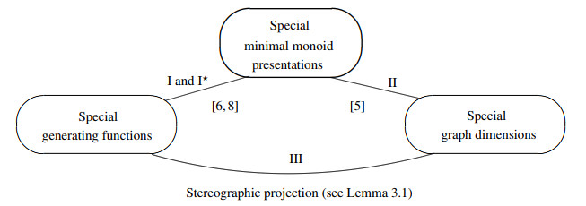
In this work, we investigated the relationship between special generating functions, such as array polynomials and graph dimensions, including metric, multiset, outer multiset, and local multiset dimensions, using minimal monoid presentations. The present paper is founded on earlier contributions and we are concerned with resolving the matching issue. In this context, our focus is on the matching between graph dimensions and generator functions, a subject that has not been examined and is alluded to in Open problem 3 in the paper by A. S. Cevik [Matching some graph dimensions with special presentations, Montes Taurus J. Pure Appl. Math., 6 (2024), 78-89]. As part of this effort, we address the characterization of graphs with infinite multiset dimensions and provide a partial classification based on outer multiset, local multiset, and metric dimensions.
- minimal presentation,
- graphs,
- metric dimension,
- multiset dimension,
- outer multiset dimension,
- local multiset dimension,
- array polynomials,
- sirling numbers
Citation: Ahmet Sinan Cevik, Ismail Naci Cangul, Yilun Shang. Matching some graph dimensions with special generating functions[J]. AIMS Mathematics, 2025, 10(4): 8446-8467. doi: 10.3934/math.2025389

Related Papers:

Abstract

In this work, we investigated the relationship between special generating functions, such as array polynomials and graph dimensions, including metric, multiset, outer multiset, and local multiset dimensions, using minimal monoid presentations. The present paper is founded on earlier contributions and we are concerned with resolving the matching issue. In this context, our focus is on the matching between graph dimensions and generator functions, a subject that has not been examined and is alluded to in Open problem 3 in the paper by A. S. Cevik [Matching some graph dimensions with special presentations, Montes Taurus J. Pure Appl. Math., 6 (2024), 78-89]. As part of this effort, we address the characterization of graphs with infinite multiset dimensions and provide a partial classification based on outer multiset, local multiset, and metric dimensions.

References

[1]	F. Ates, A. S. Cevik, Minimal but inefficient presentations for semi-direct products of finite cyclic monoids, In: Groups St. Andrews 2005, 339 (2006), 170–185.
[2]	R. Alfarisi, D. Dafik, A. I. Kristiana, I. H. Agustin, The local multiset dimension of graphs, Int. J. Eng. Technol., 8 (2019), 120–124.
[3]	I. Ali, M. Javaid, Y. Shang, Computing dominant metric dimensions of certain connected networks, Heliyon, 10 (2024), e25654.
[4]	N. H. Bong, Y. Q. Lin, Some properties of the multiset dimension of graphs, Electron. J. Graph Theory Appl., 9 (2021), 215–221.
[5]	A. S. Cevik, Matching some graph dimensions with special presentations, Montes Taurus J. Pure Appl. Math., 6 (2024), 78–89.
[6]	I. N. Cangul, A. S. Cevik, Y. Simsek, A new approach to connect algebra with analysis: relationships and applications between presentations and generating functions, Bound. Value Probl., 2013 (2013), 1–17. https://doi.org/10.1186/1687-2770-2013-51 doi: 10.1186/1687-2770-2013-51
[7]	A. S. Cevik, K. C. Das, I. N. Cangul, A. D. Maden, Minimality over free monoid presentations, Hacet. J. Math. Stat., 43 (2014), 899–913.
[8]	A. S. Cevik, K. C. Das, Y. Simsek, I. N. Cangul, Some array polynomials over special monoid presentations, Fixed Point Theory Appl., 2013 (2013), 1–14. https://doi.org/10.1186/1687-1812-2013-44 doi: 10.1186/1687-1812-2013-44
[9]	C. H. Chang, C. W. Ha, A multiplication theorem for the Lerch zeta function and explicit representations of the Bernoulli and Euler polynomials, J. Math. Anal. Appl., 315 (2006), 758–767. https://doi.org/10.1016/j.jmaa.2005.08.013 doi: 10.1016/j.jmaa.2005.08.013
[10]	R. Gil-Pons, Y. Ramirez-Cruz, R. Trujillo-Rasua, I. G. Yero, Distance-based vertex identification in graphs: the outer multiset dimension, Appl. Math. Comput., 363 (2019), 124612. https://doi.org/10.1016/j.amc.2019.124612 doi: 10.1016/j.amc.2019.124612
[11]	F. Harary, R. A. Melter, On the metric dimension of a graph, Ars Combin., 2 (1976), 191–195.
[12]	E. G. Karpuz, K. C. Das, I. N. Cangul, A. S. Cevik, A new graph based on the semi-direct product of some monoids, J. Inequal. Appl., 2013 (2013), 1–8. https://doi.org/10.1186/1029-242X-2013-118 doi: 10.1186/1029-242X-2013-118
[13]	S. Klav$\breve{{\rm{z}}}$ar, D. Kuziak, I. G. Yero, Further contributions on the outer multiset dimension of graphs, Results Math., 78 (2023), 50. https://doi.org/10.1007/s00025-022-01829-8 doi: 10.1007/s00025-022-01829-8
[14]	R. J. Lisle, P. R. Leyshon, Stereographic projection techniques for geologists and civil engineers, Cambridge University Press, 2004.
[15]	Q. M. Luo, H. M. Srivastava, Some generalizations of the Apostol-Genocchi polynomials and the Stirling numbers of the second kind, Appl. Math. Comput., 217 (2011), 5702–5728. https://doi.org/10.1016/j.amc.2010.12.048 doi: 10.1016/j.amc.2010.12.048
[16]	M. J. Mismar, D. I. Abu-Al-Nadi, T. H. Ismail, Pattern synthesis with phase-only control using array polynomial technique, In: 2007 IEEE International Conference on Signal Processing and Communications, 2007,444–447. https://doi.org/10.1109/ICSPC.2007.4728351
[17]	Y. Simsek, Generating functions for generalized Stirling type numbers, array type polynomials, Eulerian type polynomials and their applications, Fixed Point Theory Appl., 2013 (2013), 1–28. https://doi.org/10.1186/1687-1812-2013-87 doi: 10.1186/1687-1812-2013-87
[18]	P. J. Slater, Leaves of trees, In: Proceeding of the 6th Southeastern Conference on Combinatorics, Graph Theory and Computing, Congressus Numerantium, 14 (1975), 549–559.
[19]	R. Simanjuntak, P. Siagian, T. Vetrik, The multiset dimension of graphs, 2019, arXiv: 1711.00225.
[20]	E. J. W. Whittaker, C. A. Taylor, The stereographic projection, University College Cardiff Press, 1984.

Reader Comments

Your name:*

Email:*
© 2025 the Author(s), licensee AIMS Press. This is an open access article distributed under the terms of the Creative Commons Attribution License (http://creativecommons.org/licenses/by/4.0)