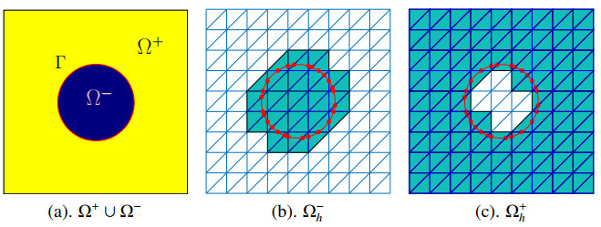
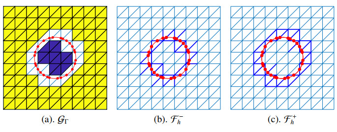
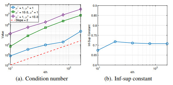
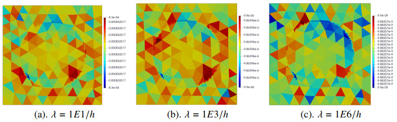
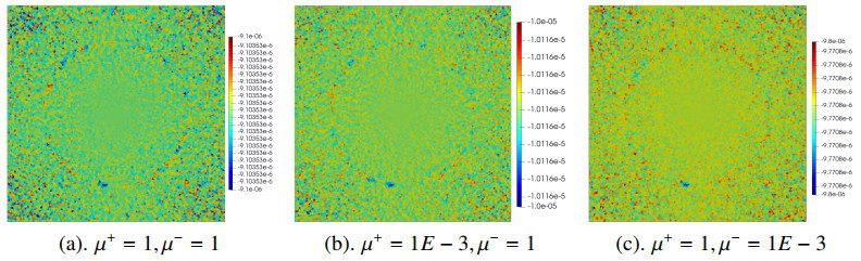
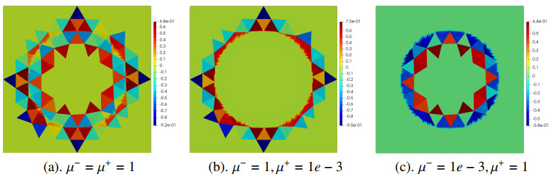
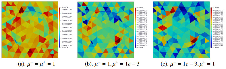
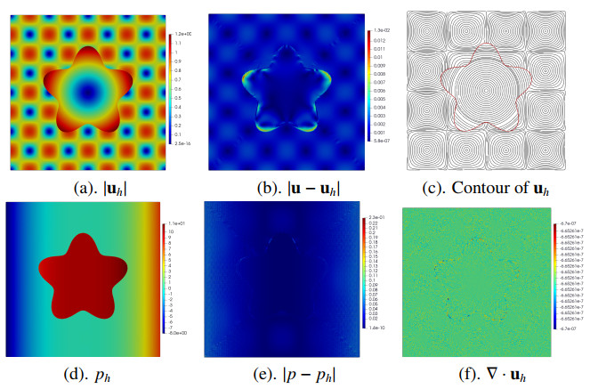
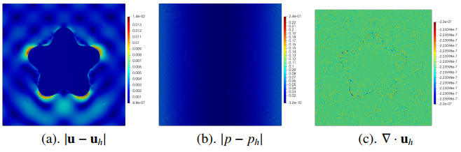
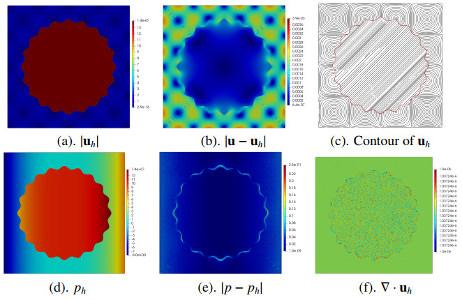
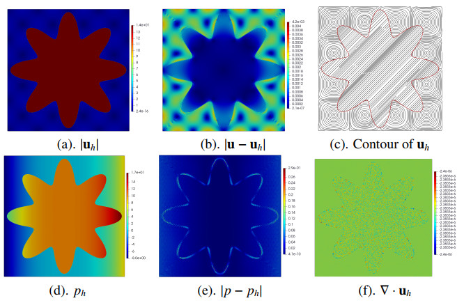
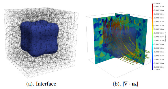
In this paper, we develop a new unfitted finite element method for the Stokes interface problem. In this method, the velocity is approximated using a piecewise linear continuous Galerkin element enriched by the lowest-order Raviart–Thomas element, while the pressure is approximated using a piecewise constant element. To construct a stable solver with an optimal convergence rate, we adopt cut finite element strategies and add ghost penalty terms for both velocity and pressure. We numerically show that the considered method achieves an optimal convergence rate as well as preserving the divergence constraint. Several benchmark problems are presented to test its stability, divergence property, and convergence performance, demonstrating the desired pressure and viscosity robustness in complex geometries, thereby outperforming other numerical methods.
Citation: Kun Wang, Lin Mu. Numerical investigation of a new cut finite element method for Stokes interface equations[J]. Electronic Research Archive, 2025, 33(4): 2503-2524. doi: 10.3934/era.2025111
In this paper, we develop a new unfitted finite element method for the Stokes interface problem. In this method, the velocity is approximated using a piecewise linear continuous Galerkin element enriched by the lowest-order Raviart–Thomas element, while the pressure is approximated using a piecewise constant element. To construct a stable solver with an optimal convergence rate, we adopt cut finite element strategies and add ghost penalty terms for both velocity and pressure. We numerically show that the considered method achieves an optimal convergence rate as well as preserving the divergence constraint. Several benchmark problems are presented to test its stability, divergence property, and convergence performance, demonstrating the desired pressure and viscosity robustness in complex geometries, thereby outperforming other numerical methods.

| [1] |
M. A. Olshanskii, A. Reusken, Analysis of a Stokes interface problem, Numer. Math., 103 (2006), 129–149. https://doi.org/10.1007/s00211-005-0646-x doi: 10.1007/s00211-005-0646-x

|
| [2] |
L. Yang, Q. Zhai, R. Zhang, The weak Galerkin finite element method for Stokes interface problems with curved interface, Appl. Numer. Math., 208 (2025), 98–122. https://doi.org/10.1016/j.apnum.2024.10.004 doi: 10.1016/j.apnum.2024.10.004
|
| [3] |
S. Claus, P. Kerfriden, A CutFEM method for two-phase flow problems, Comput. Methods Appl. Mech. Eng., 348 (2019), 185–206. https://doi.org/10.1016/j.cma.2019.01.009 doi: 10.1016/j.cma.2019.01.009
|
| [4] |
T. Frachon, S. Zahedi, A cut finite element method for incompressible two-phase Navier-Stokes flows, J. Comput. Phys., 384 (2019), 77–98. https://doi.org/10.1016/j.jcp.2019.01.028 doi: 10.1016/j.jcp.2019.01.028
|
| [5] |
H. Liu, M. Neilan, M. Olshanskii, A CutFEM divergence-free discretization for the Stokes problem, ESAIM Math. Model. Numer. Anal., 57 (2023), 143–165. https://doi.org/10.1051/m2an/2022072 doi: 10.1051/m2an/2022072
|
| [6] |
K. Wang, L. Mu, An enriched cut finite element method for Stokes interface equations, Math. Comput. Simul., 218 (2024), 644–665. https://doi.org/10.1016/j.matcom.2023.12.016 doi: 10.1016/j.matcom.2023.12.016
|
| [7] |
L. Cattaneo, L. Formaggia, G. F. Iori, A. Scotti, P. Zunino, Stabilized extended finite elements for the approximation of saddle point problems with unfitted interface, Calcolo, 52 (2015), 123–152. https://doi.org/10.1007/s10092-014-0109-9 doi: 10.1007/s10092-014-0109-9
|
| [8] |
X. He, F. Song, W. Deng, A stabilized nonconforming Nitsche's extended finite element method for Stokes interface problems, Discrete Contin. Dyn. Syst. Ser. B, 27 (2022), 2849–2871. https://doi.org/10.3934/dcdsb.2021163 doi: 10.3934/dcdsb.2021163
|
| [9] |
N. Wang, J. Chen, A nonconforming Nitsche's extended finite element method for Stokes interface problems, J. Sci. Comput., 81 (2019), 342–374. https://doi.org/10.1007/s10915-019-01019-9 doi: 10.1007/s10915-019-01019-9
|
| [10] |
S. Adjerid, N. Chaabane, T. Lin, An immersed discontinuous finite element method for Stokes interface problems, Comput. Methods Appl. Mech. Eng., 293 (2015), 170–190. https://doi.org/10.1016/j.cma.2015.04.006 doi: 10.1016/j.cma.2015.04.006
|
| [11] |
X. Chen, Z. Li, J. R. Clvarez, A direct IIM approach for two-phase Stokes equations with discontinuous viscosity on staggered grids, Comput. Fluids, 172 (2018), 549–563. https://doi.org/10.1016/j.compfluid.2018.03.038 doi: 10.1016/j.compfluid.2018.03.038
|
| [12] | Y. Chen, X. Zhang, A $P_2-P_1$ partially penalized immersed finite element method for Stokes interface problems, Int. J. Numer. Anal. Model., 18 (2021), 120–141. |
| [13] |
S. Hou, P. Song, L. Wang, H. Zhao, A weak formulation for solving elliptic interface problems without body fitted grid, J. Comput. Phys., 249 (2013), 80–95. https://doi.org/10.1016/j.jcp.2013.04.025 doi: 10.1016/j.jcp.2013.04.025
|
| [14] | J. Wang, Z. Zhang, Q. Zhuang, An immersed Crouzeix-Raviart finite element method for Navier-Stokes equations with moving interfaces, Int. J. Numer. Anal. Model., 19 (2022), 563–586. |
| [15] |
N. Zhu, H. Rui, A divergence-free Petrov-Galerkin immersed finite element method for Stokes interface problem, J. Sci. Comput., 100 (2024), 4. https://doi.org/10.1007/s10915-024-02547-9 doi: 10.1007/s10915-024-02547-9
|
| [16] |
H. Fan, Z. Tan, Novel and general discontinuity-removing PINNs for elliptic interface problems, J. Comput. Phys., 529 (2025), 113861. https://doi.org/10.1016/j.jcp.2025.113861 doi: 10.1016/j.jcp.2025.113861
|
| [17] | Y. H. Tseng, M. C. Lai, A discontinuity and cusp capturing PINN for Stokes interface problems with discontinuous viscosity and singular forces, Ann. Appl. Math., 39 (2023), 385–405. |
| [18] |
X. Li, H. Rui, A low-order divergence-free H (div)-conforming finite element method for Stokes flows, IMA J. Numer. Anal., 42 (2022), 3711–3734. https://doi.org/10.1093/imanum/drab080 doi: 10.1093/imanum/drab080
|
| [19] |
T. Frachon, P. Hansbo, E. Nilsson, S. Zahedi, A divergence preserving cut finite element method for Darcy flow, SIAM J. Sci. Comput., 46 (2024), A1793–A1820. https://doi.org/10.1137/22M149702X doi: 10.1137/22M149702X
|
| [20] |
T. Frachon, E. Nilsson, S. Zahedi, Divergence-free cut finite element methods for Stokes flow, BIT Numer. Math., 64 (2024), 39. https://doi.org/10.1007/s10543-024-01040-x doi: 10.1007/s10543-024-01040-x
|
| [21] |
P. Hansbo, M. G. Larson, S. Zahedi, A cut finite element method for a Stokes interface problem, Appl. Numer. Math., 85 (2014), 90–114. https://doi.org/10.1016/j.apnum.2014.06.009 doi: 10.1016/j.apnum.2014.06.009
|
| [22] |
Y. Sun, W. Zhao, W. Zhao, Error estimates of finite element methods for the nonlinear backward stochastic Stokes equations, CSIAM Trans. Appl. Math., 6 (2025), 31–62. https://doi.org/10.4208/csiam-am.SO-2024-0021 doi: 10.4208/csiam-am.SO-2024-0021
|
| [23] |
I. Voulis, A. Reusken, A time dependent Stokes interface problem: Well-posedness and space-time finite element discretization, ESAIM Math. Model. Numer. Anal., 52 (2018), 2187–2213. https://doi.org/10.1051/m2an/2018053 doi: 10.1051/m2an/2018053
|
| [24] |
Q. Wang, P. Huang, Y. He, The Navier-Stokes-$\omega$/Navier-Stokes-$\omega$ model for fluid-fluid interaction using an unconditionally stable finite element scheme, Int. J. Numer. Anal. Model., 22 (2025), 178–201. https://doi.org/10.4208/ijnam2025-1009 doi: 10.4208/ijnam2025-1009
|
| [25] |
L. Yang, W. Mu, H. Peng, X. Wang, The weak Galerkin finite element method for the dual-porosity-Stokes model, Int. J. Numer. Anal. Model., 21 (2024), 587–608. https://doi.org/10.4208/ijnam2024-1023 doi: 10.4208/ijnam2024-1023
|
Figures(14) / Tables(9)
Kun Wang, Lin Mu. Numerical investigation of a new cut finite element method for Stokes interface equations[J]. Electronic Research Archive, 2025, 33(4): 2503-2524. doi: 10.3934/era.2025111


 DownLoad: