FF-ResNet-DR model: a deep learning model for diabetic retinopathy grading by frequency domain attention

Chang Yu; Qian Ma; Jing Li; Qiuyang Zhang; Jin Yao; Biao Yan; Zhenhua Wang; Chang Yu; Qian Ma; Jing Li; Qiuyang Zhang; Jin Yao; Biao Yan; Zhenhua Wang

doi:10.3934/era.2025033

Electronic Research Archive

2025, Volume 33, Issue 2: 725-743. doi: 10.3934/era.2025033

Previous Article Next Article

Research article

FF-ResNet-DR model: a deep learning model for diabetic retinopathy grading by frequency domain attention

Chang Yu ¹,
Qian Ma ²,
Jing Li ³,
Qiuyang Zhang ⁴,
Jin Yao ^{4
,
,},
Biao Yan ^{5
,
,},
Zhenhua Wang ^{1
,
,}

1.
College of Information Technology, Shanghai Ocean University, Shanghai 201306, China
2.
General Hospital of Ningxia Medical University, Ningxia 750001, China
3.
Eye Institute and Department of Ophthalmology, Eye and ENT Hospital, Fudan University, Shanghai 201114, China
4.
Department of Ophthalmology and Optometry, The Affiliated Eye Hospital, Nanjing Medical University, Nanjing 210029, China
5.
Department of Ophthalmology, Shanghai General Hospital, Shanghai Jiao Tong University School of Medicine, Shanghai 200080, China

Received: 15 November 2024 Revised: 03 January 2025 Accepted: 09 January 2025 Published: 11 February 2025

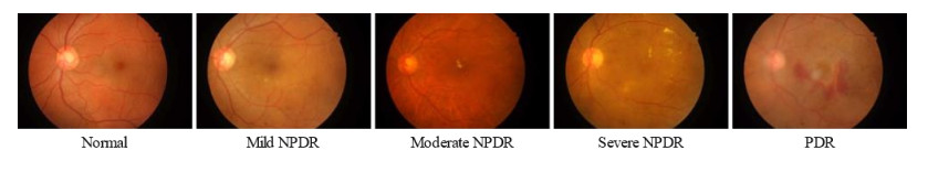
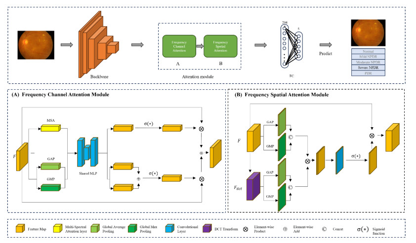
Diabetic retinopathy (DR) is a major cause of vision loss. Accurate grading of DR is critical to ensure timely and appropriate intervention. DR progression is primarily characterized by the presence of biomarkers including microaneurysms, hemorrhages, and exudates. These markers are small, scattered, and challenging to detect. To improve DR grading accuracy, we propose FF-ResNet-DR, a deep learning model that leverages frequency domain attention. Traditional attention mechanisms excel at capturing spatial-domain features but neglect valuable frequency domain information. Our model incorporates frequency channel attention modules (FCAM) and frequency spatial attention modules (FSAM). FCAM refines feature representation by fusing frequency and channel information. FSAM enhances the model's sensitivity to fine-grained texture details. Extensive experiments on multiple public datasets demonstrate the superior performance of FF-ResNet-DR compared to state-of-the-art models. It achieves an AUC of 98.1% on the Messidor binary classification task and a joint accuracy of 64.1% on the IDRiD grading task. These results highlight the potential of FF-ResNet-DR as a valuable tool for the clinical diagnosis and management of DR.
- diabetic retinopathy (DR),
- grading model,
- classification model,
- color fundus image,
- attention mechanism
Citation: Chang Yu, Qian Ma, Jing Li, Qiuyang Zhang, Jin Yao, Biao Yan, Zhenhua Wang. FF-ResNet-DR model: a deep learning model for diabetic retinopathy grading by frequency domain attention[J]. Electronic Research Archive, 2025, 33(2): 725-743. doi: 10.3934/era.2025033

Related Papers:

Abstract

Diabetic retinopathy (DR) is a major cause of vision loss. Accurate grading of DR is critical to ensure timely and appropriate intervention. DR progression is primarily characterized by the presence of biomarkers including microaneurysms, hemorrhages, and exudates. These markers are small, scattered, and challenging to detect. To improve DR grading accuracy, we propose FF-ResNet-DR, a deep learning model that leverages frequency domain attention. Traditional attention mechanisms excel at capturing spatial-domain features but neglect valuable frequency domain information. Our model incorporates frequency channel attention modules (FCAM) and frequency spatial attention modules (FSAM). FCAM refines feature representation by fusing frequency and channel information. FSAM enhances the model's sensitivity to fine-grained texture details. Extensive experiments on multiple public datasets demonstrate the superior performance of FF-ResNet-DR compared to state-of-the-art models. It achieves an AUC of 98.1% on the Messidor binary classification task and a joint accuracy of 64.1% on the IDRiD grading task. These results highlight the potential of FF-ResNet-DR as a valuable tool for the clinical diagnosis and management of DR.

References

[1]	A. O. Alamoudi, S. M. Allabun, Blood vessel segmentation with classification model for diabetic retinopathy screening, Comput. Mater. Contin., 75 (2023), 2265–2281. https://doi.org/10.32604/cmc.2023.032429 doi: 10.32604/cmc.2023.032429
[2]	J. Lo, T. Y. Timothy, D. Ma, P. Zang, J. P. Owen, Q. Zhang, et al., Federated learning for microvasculature segmentation and diabetic retinopathy classification of OCT data, Ophthalmol. Sci., 1 (2021), 100069. https://doi.org/10.1016/j.xops.2021.100069 doi: 10.1016/j.xops.2021.100069
[3]	H. Pratt, F. Coenen, D. M. Broadbent, S. P. Harding, Y. Zheng, Convolutional neural networks for diabetic retinopathy, Procedia Comput. Sci., 90 (2016), 200–205. https://doi.org/10.1016/j.procs.2016.07.014 doi: 10.1016/j.procs.2016.07.014
[4]	W. Wang, X. Li, Z. Xu, W. Yu, J. Zhao, D. Ding, et al., Learning two-stream CNN for multi-modal age-related macular degeneration categorization, IEEE J. Biomed. Health Inf., 26 (2022), 4111–4122. https://doi.org/10.1109/JBHI.2022.3171523 doi: 10.1109/JBHI.2022.3171523
[5]	Z. Wang, Y. Yin, J. Shi, W. Fang, H. Li, X. Wang, Zoom-in-net: Deep mining lesions for diabetic retinopathy detection, in Medical Image Computing and Computer Assisted Intervention−MICCAI 2017, (2017), 267–275. https://doi.org/10.1007/978-3-319-66179-7_31
[6]	L. Seoud, T. Hurtut, J. Chelbi, F. Cheriet, J. P. Langlois, Red lesion detection using dynamic shape features for diabetic retinopathy screening, IEEE Trans. Med. Imaging, 35 (2015), 1116–1126. https://doi.org/10.1109/TMI.2015.2509785 doi: 10.1109/TMI.2015.2509785
[7]	W. Zhang, J. Zhong, S. Yang, Z. Gao, J. Hu, Y. Chen, et al., Automated identification and grading system of diabetic retinopathy using deep neural networks, Knowl. Based Syst., 175 (2019), 12–25. https://doi.org/10.1016/j.knosys.2019.03.016 doi: 10.1016/j.knosys.2019.03.016
[8]	R. Zheng, L. Liu, S. Zhang, C. Zheng, F. Bunyak, R. Xu, et al., Detection of exudates in fundus photographs with imbalanced learning using conditional generative adversarial network, Biomed. Opt. Express, 9 (2018), 4863–4878. https://doi.org/10.1364/BOE.9.004863 doi: 10.1364/BOE.9.004863
[9]	X. He, Y. Deng, L. Fang, Q. Peng, Multi-modal retinal image classification with modality-specific attention network, IEEE Trans. Med. Imaging, 40 (2021), 1591–1602. https://doi.org/10.1109/TMI.2021.3059956 doi: 10.1109/TMI.2021.3059956
[10]	V. Gulshan, L. Peng, M. Coram, M. C. Stumpe, D. Wu, A. Narayanaswamy, et al., Development and validation of a deep learning algorithm for detection of diabetic retinopathy in retinal fundus photographs, JAMA, 316 (2016), 2402–2410. https://doi.org/10.1001/jama.2016.17216 doi: 10.1001/jama.2016.17216
[11]	P. Li, Y. Zhang, L. Yuan, H. Xiao, B. Lin, X. Xu, Efficient long-short temporal attention network for unsupervised video object segmentation, Pattern Recognit., 146 (2024), 110078. https://doi.org/10.1016/j.patcog.2023.110078 doi: 10.1016/j.patcog.2023.110078
[12]	P. Li, G. Zhao, J. Chen, X. Xu, Deep metric learning via group channel-wise ensemble, Knowl. Based Syst., 259 (2023), 110029. https://doi.org/10.1016/j.knosys.2022.110029 doi: 10.1016/j.knosys.2022.110029
[13]	P. Li, P. Zhang, T. Wang, H. Xiao, Time-frequency recurrent transformer with diversity constraint for dense video captioning, Inf. Process. Manage., 60 (2023), 103204. https://doi.org/10.1016/j.ipm.2022.103204 doi: 10.1016/j.ipm.2022.103204
[14]	P. Li, J. Chen, L. Yuan, X. Xu, M. Song, Triple-view knowledge distillation for semi-supervised semantic segmentation, preprint, arXiv: 2309.12557. https://doi.org/10.48550/arXiv.2309.12557
[15]	A. He, T. Li, N. Li, K. Wang, H. Fu, CABNet: Category attention block for imbalanced diabetic retinopathy grading, IEEE Trans. Med. Imaging, 40 (2020), 143–153. https://doi.org/10.1109/TMI.2020.3023463 doi: 10.1109/TMI.2020.3023463
[16]	Y. Zhou, X. He, L. Huang, L. Liu, F. Zhu, S. Cui, et al., Collaborative learning of semi-supervised segmentation and classification for medical images, in Proceedings of the IEEE/CVF Conference on Computer Vision and Pattern Recognition, IEEE, (2019), 2079–2088. https://doi.org/10.1109/CVPR.2019.00218
[17]	Y. Yang, T. Li, W. Li, H. Wu, W. Fan, W. Zhang, Lesion detection and grading of diabetic retinopathy via two-stages deep convolutional neural networks, in Lecture Notes in Computer Science, Springer, (2017), 533–540. https://doi.org/10.1007/978-3-319-66179-7_61
[18]	X. Li, X. Hu, L. Yu, L. Zhu, C. W. Fu, P. A. Heng, CANet: Cross-disease attention network for joint diabetic retinopathy and diabetic macular edema grading, IEEE Trans. Med. Imaging, 39 (2019), 1483–1493. https://doi.org/10.1109/TMI.2019.2951844 doi: 10.1109/TMI.2019.2951844
[19]	Z. Qin, P. Zhang, F. Wu, X. Li, Fcanet: Frequency channel attention networks, in Proceedings of the IEEE/CVF International Conference on Computer Vision (ICCV), IEEE, (2021), 783–792. https://doi.org/10.1109/ICCV48922.2021.00082
[20]	T. Zhou, Z. Ma, Q. Wen, X. Wang, L. Sun, R. Jin, Fedformer: Frequency enhanced decomposed transformer for long-term series forecasting, in Proceedings of the 39th International Conference on Machine Learning, PMLR, (2022), 27268–27286. https://doi.org/10.48550/arXiv.2201.12740
[21]	R. Sun, Y. Li, T. Zhang, Z. Mao, F. Wu, Y. Zhang, Lesion-aware transformers for diabetic retinopathy grading, in 2021 IEEE/CVF Conference on Computer Vision and Pattern Recognition (CVPR), IEEE, (2021), 10938–10947. https://doi.org/10.1109/CVPR46437.2021.01079
[22]	E. Decencière, X. Zhang, G. Cazuguel, B. Lay, B. Cochener, C. Trone, et al., Feedback on a publicly distributed image database: The Messidor database, Image Anal. Stereol., (2014), 231–234. https://doi.org/10.5566/ias.1155 doi: 10.5566/ias.1155
[23]	M. M. Farag, M. Fouad, A. T. Abdel-Hamid, Automatic severity classification of diabetic retinopathy based on densenet and convolutional block attention module, IEEE Access, 10 (2022), 38299–38308. https://doi.org/10.1109/ACCESS.2022.3165193 doi: 10.1109/ACCESS.2022.3165193
[24]	P. Porwal, S. Pachade, R. Kamble, M. Kokare, G. Deshmukh, V. Sahasrabuddhe, et al., Indian diabetic retinopathy image dataset (IDRiD): A database for diabetic retinopathy screening research, Data, 3 (2018), 25. https://doi.org/10.3390/data3030025 doi: 10.3390/data3030025
[25]	T. Li, Y. Gao, K. Wang, S. Guo, H. Liu, H. Kang, Diagnostic assessment of deep learning algorithms for diabetic retinopathy screening, Inf. Sci., 501 (2019), 511–522. https://doi.org/10.1016/j.ins.2019.06.011 doi: 10.1016/j.ins.2019.06.011
[26]	K. He, X. Zhang, S. Ren, J. Sun, Deep residual learning for image recognition, in Proceedings of the IEEE Conference on Computer Vision and Pattern Recognition (CVPR), IEEE, (2016), 770–778. https://doi.org/10.1109/CVPR.2016.90
[27]	J. Cohen, Weighted kappa: Nominal scale agreement provision for scaled disagreement or partial credit, Psychol. Bull., 70 (1968), 213. https://doi.org/10.1037/h0026256 doi: 10.1037/h0026256
[28]	M. Sokolova, N. Japkowicz, S. Szpakowicz, Beyond accuracy, F-score and ROC: A family of discriminant measures for performance evaluation, in Australasian Joint Conference on Artificial Intelligence, (2006), 1015–1021. https://doi.org/10.1007/11941439_114
[29]	S. Woo, J. Park, J. Y. Lee, I. S. Kweon, Cbam: Convolutional block attention module, preprint, arXiv: 1807.06521. https://doi.org/10.48550/arXiv.1807.06521
[30]	N. Ahmed, T. Natarajan, K. R. Rao, Discrete cosine transform, IEEE Trans. Comput., 100 (1974), 90–93. https://doi.org/10.1109/T-C.1974.223784 doi: 10.1109/T-C.1974.223784
[31]	X. Liu, W. Chi, A cross-lesion attention network for accurate diabetic retinopathy grading with fundus images, IEEE Trans. Instrum. Meas., 72 (2023), 1–12. https://doi.org/10.1109/TIM.2023.3322497 doi: 10.1109/TIM.2023.3322497
[32]	R. R. Selvaraju, M. Cogswell, A. Das, R. Vedantam, D. Parikh, D. Batra, Grad-CAM: Visual explanations from deep networks via gradient-based localization, in 2017 IEEE International Conference on Computer Vision (ICCV), (2017), 618–626, https://doi.org/10.1109/ICCV.2017.74

Reader Comments

Your name:*

Email:*
© 2025 the Author(s), licensee AIMS Press. This is an open access article distributed under the terms of the Creative Commons Attribution License (http://creativecommons.org/licenses/by/4.0)