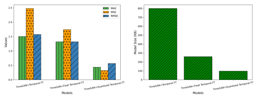
The deployment of real-time sensor calibration models for air pollution monitoring on resource-constrained Industrial Internet of Things (IIoT) edge devices presents significant challenges due to the computational complexity and memory requirements of deep learning models. This paper addressed these challenges by proposing a time-series-generative approach that integrated model quantization, generative artificial intelligence (AI), and temporal deep learning architectures to ensure efficient deployment. Specifically, we introduced a TimeGAN-augmented temporal fusion transformer (TFT) model optimized for edge devices. By leveraging model quantization, the approach reduces the memory footprint and computational demands of the model without compromising calibration accuracy. Furthermore, the integration of generative adversarial networks (GANs) enhances the robustness of the model by generating high-quality synthetic time-series data, compensating for sparse or noisy sensor readings. This ability to generate synthetic data mirrors the real sensor trends, ensuring reliable model performance even in data-limited environments. A comprehensive evaluation of the proposed model, comparing its performance against both float and quantized versions, demonstrates the effectiveness of the TimeGAN-augmented quantized TFT. This model achieves a significant 88% reduction in size (from 800.04 KB to 97.34 KB) while maintaining excellent predictive performance, evidenced by a mean squared error (MSE) of 0.3212 and a mean absolute error (MAE) of 0.4375. Additionally, the TimeGAN-augmented Float TFT model emerges as a strong contender for real-time applications, offering an optimal balance between inference speed and accuracy, with a rapid inference time of 23.4 ms, making it ideal for real-time pollution monitoring.
Citation: Shagufta Henna, Mohammad Amjath, Asif Yar. Time-generative AI-enabled temporal fusion transformer model for efficient air pollution sensor calibration in IIoT edge environments[J]. AIMS Environmental Science, 2025, 12(3): 526-556. doi: 10.3934/environsci.2025024
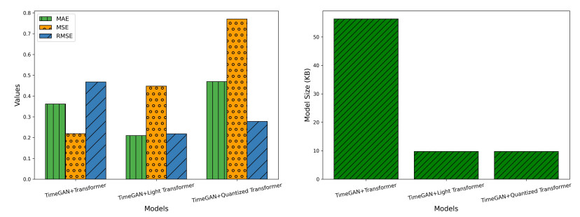
The deployment of real-time sensor calibration models for air pollution monitoring on resource-constrained Industrial Internet of Things (IIoT) edge devices presents significant challenges due to the computational complexity and memory requirements of deep learning models. This paper addressed these challenges by proposing a time-series-generative approach that integrated model quantization, generative artificial intelligence (AI), and temporal deep learning architectures to ensure efficient deployment. Specifically, we introduced a TimeGAN-augmented temporal fusion transformer (TFT) model optimized for edge devices. By leveraging model quantization, the approach reduces the memory footprint and computational demands of the model without compromising calibration accuracy. Furthermore, the integration of generative adversarial networks (GANs) enhances the robustness of the model by generating high-quality synthetic time-series data, compensating for sparse or noisy sensor readings. This ability to generate synthetic data mirrors the real sensor trends, ensuring reliable model performance even in data-limited environments. A comprehensive evaluation of the proposed model, comparing its performance against both float and quantized versions, demonstrates the effectiveness of the TimeGAN-augmented quantized TFT. This model achieves a significant 88% reduction in size (from 800.04 KB to 97.34 KB) while maintaining excellent predictive performance, evidenced by a mean squared error (MSE) of 0.3212 and a mean absolute error (MAE) of 0.4375. Additionally, the TimeGAN-augmented Float TFT model emerges as a strong contender for real-time applications, offering an optimal balance between inference speed and accuracy, with a rapid inference time of 23.4 ms, making it ideal for real-time pollution monitoring.

| [1] |
Yar A, Henna S, McAfee M, et al. (2023) Air Pollution Monitoring Using Online Recurrent Extreme Learning Machine. 31st Irish Conference on Artificial Intelligence and Cognitive Science (AICS) 2023: 1–6. https://doi.org/10.1109/AICS60730.2023.10470534 doi: 10.1109/AICS60730.2023.10470534

|
| [2] |
Alsamrai O, Redel-Macias MD, Pinzi S, et al. (2024) A systematic review for indoor and outdoor air pollution monitoring systems based on Internet of Things. Sustainability 16: 4353. https://doi.org/10.3390/su16114353 doi: 10.3390/su16114353
|
| [3] |
Castell N, Dauge FR, Schneider P, et al. (2017) Can commercial low-cost sensor platforms contribute to air quality monitoring and exposure estimates? Environ Int 99: 293-302. https://doi.org/10.1016/j.envint.2016.12.007 doi: 10.1016/j.envint.2016.12.007
|
| [4] |
Wang Z, Zhang Z, Wang Z, et al. (2024) A novel intelligent indoor fire and combustibles detection method based on multi-channel transfer learning strategy with acoustic signals. Process Safety and Environmental Protection 189: 1217–1225. https://doi.org/10.1016/j.psep.2024.06.020 doi: 10.1016/j.psep.2024.06.020
|
| [5] |
Henna S, Yar A, Saheed K, et al. (2023) Wireless Sensor Networks Calibration using Attention-based Gated Recurrent Units for Air Pollution Monitoring. IEEE International Conference on Big Data (BigData) 2023: 3779–3784. https://doi.org/10.1109/BigData59044.2023.10386318 doi: 10.1109/BigData59044.2023.10386318
|
| [6] |
Maag B, Zhou Z, Saukh O, et al. (2017) SCAN: Multi-Hop Calibration for Mobile Sensor Arrays. ACM Trans Sens Netw 1. https://doi.org/10.1145/3090084 doi: 10.1145/3090084
|
| [7] |
Feng H, Xu C, Jin B, et al. (2024) A Deployment Optimization for Wireless Sensor Networks Based on Stacked Auto Encoder and Probabilistic Neural Network. Digital Communications and Networks https://doi.org/10.1016/j.dcan.2024.06.003 doi: 10.1016/j.dcan.2024.06.003
|
| [8] |
Yar A, Henna S, McAfee M, et al. (2023) Extreme Learning Machines for Calibration and Prediction in Wireless Sensor Networks: Advancing Environmental Monitoring Efficiency. 31st Irish Conference on Artificial Intelligence and Cognitive Science (AICS) 2023: 1–4. https://doi.org/10.1109/AICS60730.2023.10470795 doi: 10.1109/AICS60730.2023.10470795
|
| [9] |
Singh A, Chatterjee K, Satapathy SC (2022) An edge based hybrid intrusion detection framework for mobile edge computing. Complex Intell Syst 8: 3719-3746. https://doi.org/10.1007/s40747-021-00498-4 doi: 10.1007/s40747-021-00498-4
|
| [10] |
Idrissi I, Azizi M, Moussaoui O (2022) A Lightweight Optimized Deep Learning-based Host-Intrusion Detection System Deployed on the Edge for IoT. International Journal of Computing and Digital Systems 11: 209-216. https://doi.org/10.12785/ijcds/110117 doi: 10.12785/ijcds/110117
|
| [11] | Yandouzi M, Grari M, Idrissi I, et al. (2022) Review on forest fires detection and prediction using deep learning and drones. Journal of Theoretical and Applied Information Technology 100: 4565-4576. |
| [12] | Abusitta A, Carvalho GHS, Wahab OA, et al. (2022) Deep learning-enabled anomaly detection for IoT systems. Internet Things 21: 100656. https://api.semanticscholar.org/CorpusID: 253431423 |
| [13] |
Aversano L, Bernardi ML, Cimitile M, et al. (2021) Effective anomaly detection using deep learning in IoT systems. Wireless Communications and Mobile Computing 2021: 9054336. https://doi.org/10.1155/2021/9054336 doi: 10.1155/2021/9054336
|
| [14] |
Ahmad Z, Shahid Khan A, Nisar K, et al. (2021) Anomaly Detection Using Deep Neural Network for IoT Architecture. Applied Sciences 11: 7050. https://doi.org/10.3390/app11157050 doi: 10.3390/app11157050
|
| [15] | Konaite M, Owolawi PA, Mapayi T, et al. (2021) Smart hat for the blind with real-time object detection using Raspberry Pi and TensorFlow Lite. Proceedings of the International Conference on Artificial Intelligence and its Applications ISBN 9781450385756. https://doi.org/10.1145/3487923.3487929 |
| [16] |
Sharma K, Eskicioglu R (2022) Deep learning-based ECG classification on Raspberry Pi using a TensorFlow Lite model based on PTB-XL dataset. International Journal of Artificial Intelligence & Applications 13: 55-66. https://doi.org/10.5121/ijaia.2022.1340455 doi: 10.5121/ijaia.2022.1340455
|
| [17] |
Rokh B, Azarpeyvand A, Khanteymoori A (2023) A comprehensive survey on model quantization for deep neural networks in image classification. ACM Computing Surveys 14. https://doi.org/10.1145/3623402 doi: 10.1145/3623402
|
| [18] | Phuong M, Lampert C (2019) Towards understanding knowledge distillation. Proceedings of the 36th International Conference on Machine Learning 97: 5142–5151. PMLR. https://proceedings.mlr.press/v97/phuong19a.html |
| [19] |
Yang L, He Z, Fan D (2020) Harmonious coexistence of structured weight pruning and ternarization for deep neural networks. Proceedings of the AAAI Conference on Artificial Intelligence 34: 6623–6630. https://doi.org/10.1609/aaai.v34i04.6138 doi: 10.1609/aaai.v34i04.6138
|
| [20] | TensorFlow Lite. Ultralytics, 2024. Available from: https://developers.googleblog.com/en/tensorflow-lite-is-now-litert |
| [21] |
Sun C, Li J, Sulaiman R, et al. (2023) Air Quality Prediction and Multi-Task Offloading based on Deep Learning Methods in Edge Computing. Journal of Grid Computing 21. https://doi.org/10.1007/s10723-023-09671-0 doi: 10.1007/s10723-023-09671-0
|
| [22] | Yoon J, Jarrett D, van der Schaar M (2019) Time-series Generative Adversarial Networks. In: Neural Information Processing Systems, 2019. https://proceedings.neurips.cc/paper_files/paper/2019/file/c9efe5f26cd17ba6216bbe2a7d26d490-Paper.pdf |
| [23] |
Kursa MB, Jankowski A, Rudnicki WR (2010) Boruta – A System for Feature Selection. Fundamenta Informaticae 101: 271–285. https://doi.org/10.3233/FI-2010-288 doi: 10.3233/FI-2010-288
|
| [24] |
Moursi AS, El-Fishawy N, Djahel S, et al. (2021) An IoT enabled system for enhanced air quality monitoring and prediction on the edge. Complex and Intelligent Systems 7: 2923–2947. https://doi.org/10.1007/s40747-021-00476-w doi: 10.1007/s40747-021-00476-w
|
| [25] |
Felici-Castell S, Segura-Garcia J, Perez-Solano JJ, et al. (2023) AI-IoT low-cost pollution-monitoring sensor network to assist citizens with respiratory problems. Sensors 23. https://doi.org/10.3390/s23239585 doi: 10.3390/s23239585
|
| [26] | Li S, Jin X, Xuan Y, et al. (2019) Enhancing the locality and breaking the memory bottleneck of Transformer on time series forecasting. arXiv abs/1907.00235. https://api.semanticscholar.org/CorpusID: 195766887 |
| [27] |
Gong L, Chen Y (2024) Machine learning-enhanced IoT and wireless sensor networks for predictive analysis and maintenance in wind turbine systems. Int J Intell Netw 5: 133-144. https://doi.org/10.1016/j.ijin.2024.02.002 doi: 10.1016/j.ijin.2024.02.002
|
| [28] |
Aggarwal A, Toshniwal D (2021) A hybrid deep learning framework for urban air quality forecasting. J Clean Prod 329: Article ID 129660. https://doi.org/10.1016/j.jclepro.2021.129660 doi: 10.1016/j.jclepro.2021.129660
|
| [29] |
Wardana INK, Gardner JW, Fahmy SA (2021) Optimising deep learning at the edge for accurate hourly air quality prediction. Sensors (Switzerland) 21: 1-28. https://doi.org/10.3390/s21041064 doi: 10.3390/s21041064
|
| [30] |
Hu Y, Cao N, Guo W, et al. (2024) FedDeep: A federated deep learning network for edge-assisted multi-urban PM2.5 forecasting. Appl Sci (Switzerland) 14: Article ID 1979. https://doi.org/10.3390/app14051979 doi: 10.3390/app14051979
|
| [31] |
Koziel S, Pietrenko-Dabrowska A, Wojcikowski M, et al. (2024) High-performance machine-learning-based calibration of low-cost nitrogen dioxide sensor using environmental parameter differentials and global data scaling. Sci Rep 14: 26120. https://doi.org/10.1038/s41598-024-77214-y doi: 10.1038/s41598-024-77214-y
|
| [32] |
Yu H, Li Q, Geng YA, et al. (2020) AirNet: A calibration model for low-cost air monitoring sensors using dual sequence encoder networks. AAAI 34: Article ID 5464. https://doi.org/10.1609/aaai.v34i01.5464 doi: 10.1609/aaai.v34i01.5464
|
| [33] | Yar A, Henna S, McAfee M, et al. (2024) Accelerating deep learning for self-calibration in large-scale uncontrolled wireless sensor networks for environmental monitoring. Proc 35th Irish Syst Signals Conf (ISSC 2024), Article ID 10603082. https://doi.org/10.1109/ISSC61953.2024.10603082 |
| [34] |
Schmitz S, Towers S, Villena G, et al. (2021) Unravelling a black box: An open-source methodology for the field calibration of small air quality sensors. Atmos Meas Tech 14: 7221-7241. https://doi.org/10.5194/amt-14-7221-2021 doi: 10.5194/amt-14-7221-2021
|
| [35] |
Wang G, Yu C, Guo K, et al. (2024) Research of low-cost air quality monitoring models with different machine learning algorithms. Atmos Meas Tech 17: 181-196. https://doi.org/10.5194/amt-17-181-2024 doi: 10.5194/amt-17-181-2024
|
| [36] |
Rahardja U, Aini Q, Manongga D, et al.(2023) Enhancing machine learning with low-cost PM 2.5 air quality sensor calibration using image processing. APTSI Trans Manag (ATM) 7: 194-202. https://doi.org/10.33050/atm.v7i3.2062 doi: 10.33050/atm.v7i3.2062
|
| [37] |
Price I, Sanchez-Gonzalez A, Alet F, et al. (2024) Probabilistic weather forecasting with machine learning. Nature https://doi.org/10.1038/s41586-024-08252-9 doi: 10.1038/s41586-024-08252-9
|
| [38] | Li L, Carver R, Lopez-Gomez I, et al. (2023) SEEDS: Emulation of weather forecast ensembles with diffusion models. arXiv abs/2306.14066. https://api.semanticscholar.org/CorpusID: 259252403 |
| [39] | Wang Z, Chen C, Zeng Y, et al. (2023) Where did I come from? Origin attribution of AI-generated images. Advances in Neural Information Processing Systems 36: 74478–74500. https://proceedings.neurips.cc/paper_files/paper/2023/file/ebb4c188fafe7da089b41a9f615ad84d-Paper-Conference.pdf |
| [40] |
Tan K, Chen J, Wang D (2019) Gated Residual Networks with Dilated Convolutions for Monaural Speech Enhancement. IEEE/ACM Trans Audio Speech Lang Process 27: 189–198. https://doi.org/10.1109/TASLP.2018.2876171 doi: 10.1109/TASLP.2018.2876171
|
| [41] |
Barcelo-Ordinas JM, Ferrer-Cid P, Garcia-Vidal J, et al. (2021) H2020 project CAPTOR dataset: Raw data collected by low-cost MOX ozone sensors in a real air pollution monitoring network. Data in Brief 36: 107127. https://doi.org/10.1016/j.dib.2021.107127 doi: 10.1016/j.dib.2021.107127
|
| [42] |
Barcelo-Ordinas JM, Ferrer-Cid P, Garcia-Vidal J, et al. (2019) Distributed multi-scale calibration of low-cost ozone sensors in wireless sensor networks. Sensors 19:2503. https://doi.org/10.3390/s19112503 doi: 10.3390/s19112503
|
| [43] |
Gonsek A, Jeschke M, Rönnau S, et al. (2021) From Paths to Routes: A Method for Path Classification. Frontiers in Behavioral Neuroscience 14:610560. 10.3389/fnbeh.2020.610560 doi: 10.3389/fnbeh.2020.610560
|
| [44] | Bai S, Kolter JZ, Koltun V (2018) An Empirical Evaluation of Generic Convolutional and Recurrent Networks for Sequence Modeling. International Conference on Machine Learning (ICML). |
| [45] | Lea C, Flynn MD, Vidal R, et al. (2017) Temporal Convolutional Networks for Action Segmentation and Detection. IEEE Conference on Computer Vision and Pattern Recognition (CVPR). |
| [46] | Oord AV, Dieleman S, Zen H, et al. (2016) WaveNet: A Generative Model for Raw Audio. arXiv preprint arXiv: 1609.03499 |
| [47] | Chung J, Kastner K, Dinh L, et al. (2015) Recurrent Latent Variable Models for Sequential Data. Advances in Neural Information Processing Systems (NeurIPS). |
| [48] | Fraccaro M, Sønderby SK, Paquet U, et al. (2016) Sequential Neural Models with Stochastic Layers. Advances in Neural Information Processing Systems (NeurIPS). |
| [49] | Walker J, Doersch C, Gupta A, et al. (2016) The Uncertainty in Action: Unsupervised Action Prediction with Variational Autoencoders. European Conference on Computer Vision (ECCV). |
Figures(15) / Tables(4)

Shagufta Henna, Mohammad Amjath, Asif Yar. Time-generative AI-enabled temporal fusion transformer model for efficient air pollution sensor calibration in IIoT edge environments[J]. AIMS Environmental Science, 2025, 12(3): 526-556. doi: 10.3934/environsci.2025024


 DownLoad: